

- Every town is bound to the surrounding countryside, over which its economic, social and cultural influence spreads. The area so linked to a city is its sphere of urban influence.
- Within it the city supplies goods and services and receives labour, food, raw materials and other inputs. The area is functionally and economically integrated with the city through a two-way flow.
- Its size depends on the number and order of the city’s functions, and its boundary is fixed where a rival centre’s pull becomes stronger. Delimiting that boundary is a core problem of urban and regional planning.
Concept of the Sphere of Urban Influence

Meaning and Terminology
- Definition: the sphere of urban influence is the catchment area of a city from which it draws products, labour and services and to which it provides goods and services. It is a functional region with two-way linkages.
- Older accounts credit the term sphere of influence to Ray M. Northam, with support from Harold Carter.
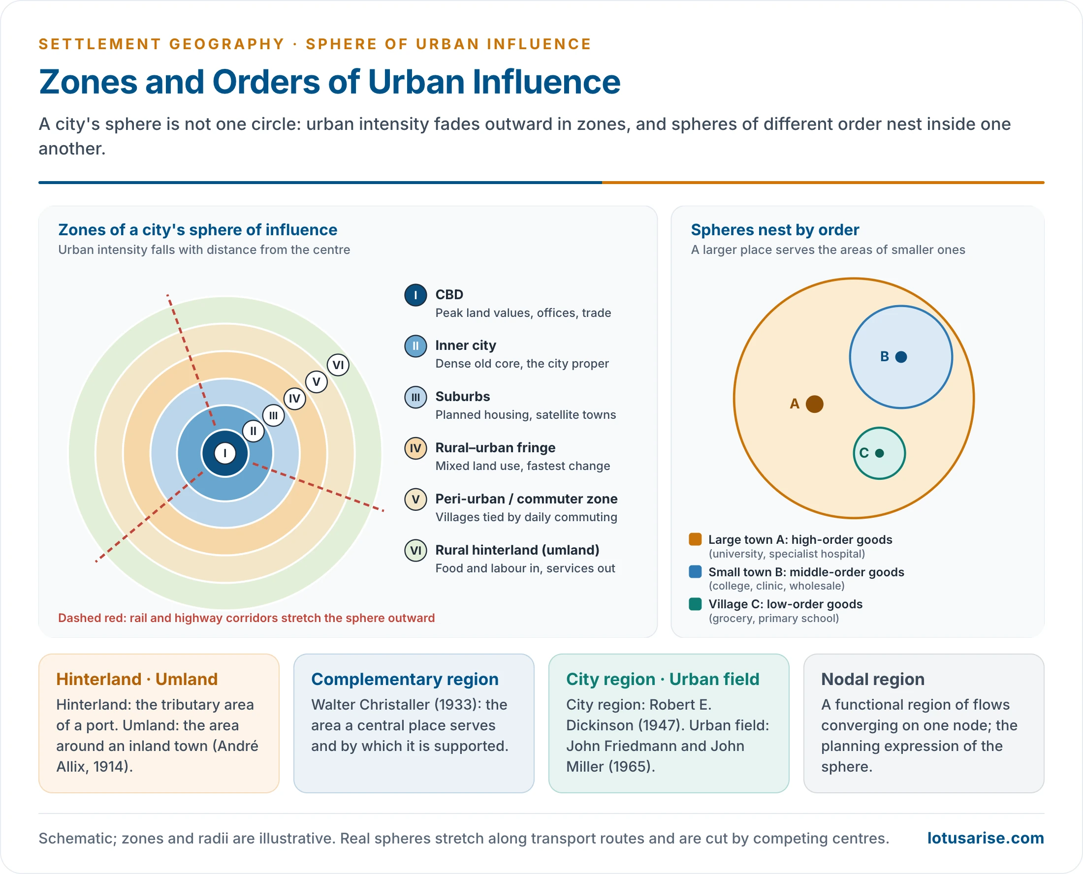
- Roots in central place theory: in Walter Christaller’s central place theory (1933), the area served by a central place is its complementary region, the area whose population supports the services the centre offers.
- On his uniform plain these regions are hexagons nested in a hierarchy of urban settlements: each higher-order centre serves the complementary regions of several lower-order ones.
- The sphere of influence goes beyond the purely economic service area. It covers all forms of interaction between a city and its region:
- commuting and migration;
- newspaper circulation and media reach;
- hospital, school and college catchments;
- retail trade areas and wholesale markets;
- bus and rail service zones and administrative jurisdictions.
- Umland (German, “the land around”):
- The French geographer André Allix (1914) gave the word its geographical meaning: the economic realm of an inland town, as opposed to the hinterland of a port.
- It was later taken up by American geographers, for example Derwent Whittlesey (1937) in his study of Kano.
- Scandinavian and German geographers use the term widely.
- Hinterland: the tributary region of a port, from which it draws exports and to which it distributes imports. Today the term is used loosely for any urban service area.
- City region: the largest possible sphere, over which the city provides its highest-range goods and services. The term was developed by Robert E. Dickinson to describe the same relationship on a much larger scale.
- Urban field: John Friedmann and John Miller (1965) used it for the wide zone, beyond the commuting belt, within which the daily and weekly life of an urbanised population takes place.
- Nodal region: a functional region of flows of goods, people, money and information converging on one node. It is the planning-region expression of the sphere.
- General principles:
- Every urban centre, whatever its size or function, has a region of influence.
- The intensity of influence decreases with distance from the core (distance decay).
- A larger population means more numerous and higher-order functions, and so a larger sphere.
- The sphere is proportional to the number and volume of services. Mumbai’s sphere is larger than Lucknow’s because Mumbai provides more and higher services.
- Fast transport and communication enlarge the sphere.
- Spheres range in scale from a few kilometres for a village market to the whole nation for a capital, and to the world for global cities such as London, New York and Tokyo.
- Range of goods and services: the distance a rational consumer will travel to obtain them from the city.
- A person in Chennai buys a smartphone in Chennai itself but must go to Delhi for the Supreme Court. Each function has its own range, and so its own sphere.
| Term | Origin | Applied to | Emphasis |
|---|---|---|---|
| Hinterland | German, “land behind” | Ports | Trade flows through the port |
| Umland | German, “land around”; André Allix (1914) | Inland towns | All-round economic realm |
| Complementary region | Walter Christaller (1933) | Central places | Area supporting central functions |
| City region | Robert E. Dickinson (1947) | Large cities | Largest functional region; planning unit |
| Urban field | Friedmann and Miller (1965) | Metropolises | Daily and weekly life space |
| Sphere of influence | General usage | Any town | All forms of urban dominance |
Structure of the Sphere: Influence, Dominance, Competition and City Region
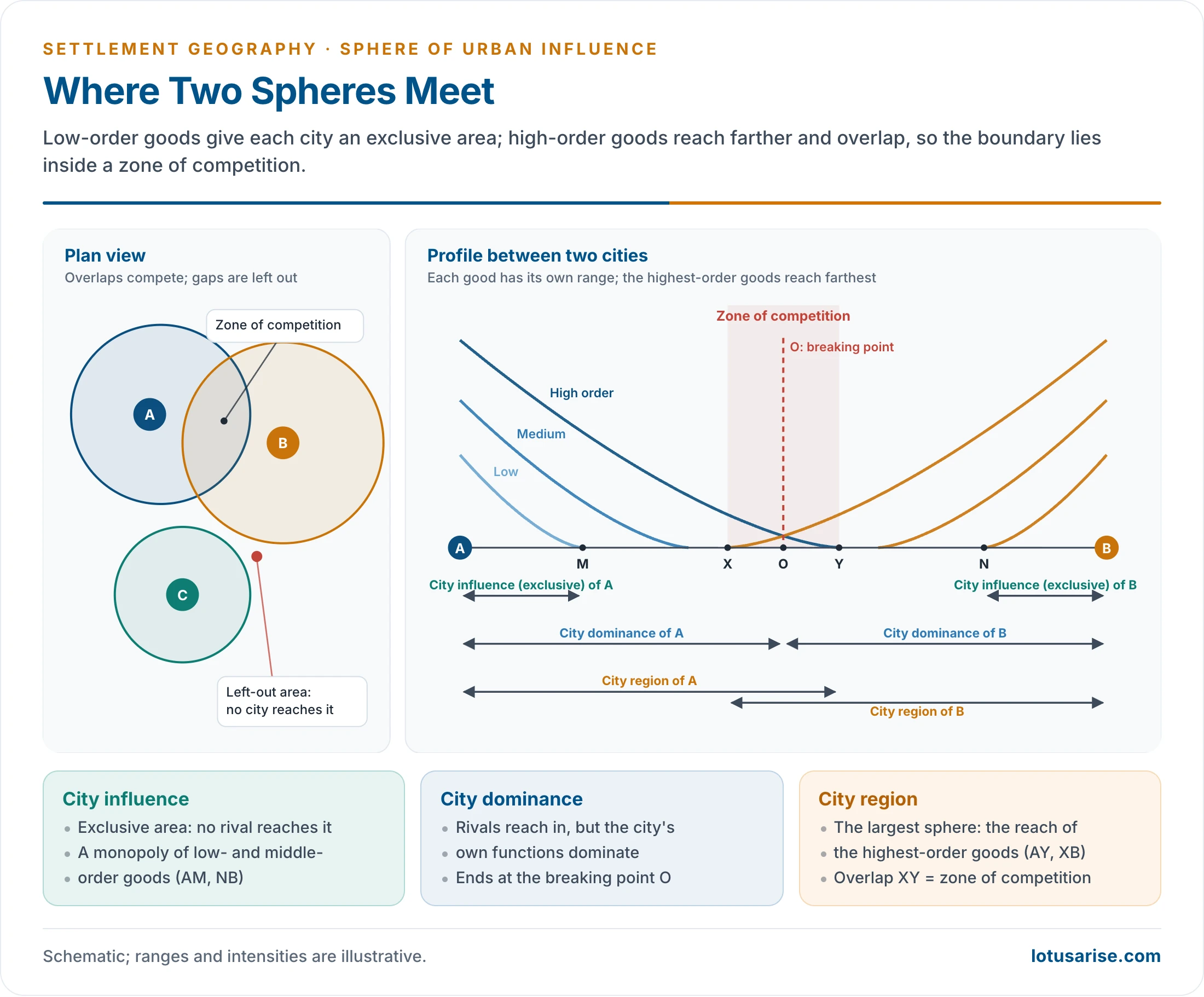
- When two cities A and B lie near each other, the area between them divides into distinct parts:
- City influence (exclusive area): the area where the city’s influence extends without competition. The city holds a monopoly, usually in low- and medium-order goods and services. In the profile these are AM for A and NB for B.
- City dominance: the area where the city competes with others but its own functions dominate. It extends to the breaking point O.
- Zone of competition: the overlap or interface where two or more cities supply goods and services. The boundary of each city’s sphere is fixed inside this zone.
- City region: the largest extent of the sphere, set by the range of the highest-order goods: AY for A and XB for B.
- City regions are identified by the intensity and magnitude of their functions, and here the distance-decay law operates.
- The structure depends on the centrality (demand) of goods and services and their characteristic range (distance).
- Gaps between spheres form left-out areas that no city serves well. They are common in hilly, tribal and border tracts.
Threshold and Range: the Two Determinants of Size
- Two concepts of central place theory set the size of a city’s sphere:
- Threshold population: the minimum number of consumers needed to support a good or service. A grocery may survive on three villages; a designer jeweller needs a whole metropolitan market. Higher-order functions have higher thresholds and larger spheres.
- Range of a good: the maximum distance consumers will travel for it. The range of milk or bread is short; that of cardiac surgery or university education very long. The range sets the outer limit of the sphere for that function.
- The sphere lies between the threshold and the range. It must hold the threshold population but cannot extend beyond the range.
- A city provides many goods with different thresholds and ranges. Its sphere is therefore a nested set of overlapping zones, not a single circle.
The City Region: Dickinson’s Framework (1947)
- Robert E. Dickinson, in City Region and Regionalism (1947), first described and theorised the city region systematically.
- Around every city lies a hinterland with which it interacts intensely and for which it is the focal point.
- Routes binding the area to the city create common interests and common organisations.
- The regional character is strongest near the focus and fades outward, dissipating at the periphery.
- The city region is a functional region, shaped by flows of people, goods, information and services, not by administrative boundaries.
- There is no sharp boundary, only a gradual transition.
- Delimitation is complex and its criteria vary between regions: telephone connections, newspaper circulation, the commuting limit, local bus routes, retail areas, hospital catchments and daily markets.
- Rapid urbanisation produced continuous built-up areas where city regions overlap and merge into conurbations.
- In planning, the city region is the logical basis of metropolitan planning regions. Planning cannot stop at the municipal boundary.
Breaking Down of Walls: the Transition Zone
- In walled cities the wall was a sharp line between urban and rural.
- With the breaking down of walls that line disappeared. It was replaced by a transition zone known as the rural–urban fringe, peri-urban zone or suburban zone.
- The zone shows characteristics of both urban and rural life: built-up areas beside open spaces and farms.
- Two relationships explain this zone:
- A growing city expands at the expense of the countryside. Urban characteristics decrease with distance from the centre.
- The city as a central place generates interaction with its surroundings. More interaction brings commercialisation, better communications and higher density.
- Either way, fringe villages urbanise and finally merge with the city. The change is first de facto and later de jure, when municipal boundaries are extended.
Zones Within the Sphere
- The sphere is organised into zones of decreasing urban intensity outward from the centre:
- City core / CBD: maximum land values, commercial intensity and functional concentration. It is the focal point of transport routes, crowded by day and dominated by high-rise offices.
- Inner city: dense mixed residential, commercial and light-industrial uses. In Indian cities it holds the old mohallas, artisan quarters and inner markets; this is the city proper under the municipal body.
- Suburban zone: planned residential areas with good road and rail links to the CBD and small local service centres. Residents commute for tertiary and quaternary work; satellite townships belong here.
- Rural–urban fringe: mixed land use with urban and rural features side by side. Farmland is interspersed with colonies, informal settlements and industrial estates, and administration is part urban, part panchayat. It is the zone of fastest, least controlled change.
- Peri-urban or commuter zone: essentially rural but with many residents commuting to the city. Influence is felt through roads, railways, land prices and the city’s pull on farm produce. Faster transport extends this zone considerably.
- Beyond the fringe, the urban shadow is an area that looks rural but is owned, commuted from and speculated on by city dwellers.
- Rural hinterland or service area: the wider area that sends farm produce, raw materials and labour to the city and receives higher-order services: specialist hospitals, universities, wholesale markets and banks. Its outer limit is where another city’s influence becomes stronger.
Factors Shaping the Size and Shape of the Sphere
- Size and functional complexity of the city: more and higher-order functions widen the sphere.
- Transport and communication: highways, railways and rapid transit stretch the sphere along their lines, giving it a star shape.
- Competition from neighbouring centres, which truncates the sphere on the side facing a rival.
- Physical barriers: rivers, hills, forests and deserts.
- Administrative and political boundaries: a State or international border cuts flows.
- Socio-economic status of consumers: richer households bypass small centres for distant high-order ones.
- Technology: online retail, digital payments and telemedicine weaken distance decay for some goods. They also strengthen the national reach of the largest cities.
- History and policy: a capital, port or cantonment acquires administrative and trade links that outlast the original reason; planning decisions on industry, universities and hospitals redraw spheres.
Significance of Studying the Sphere
- Regional planning: the sphere is the natural unit for metropolitan and district planning, linking a city with the villages and towns that depend on it.
- Location of services: hospitals, colleges, banks, warehouses and markets are placed by catchment, so that thresholds are met and no area is left out.
- Administrative reorganisation: district, division and municipal limits can be redrawn to follow functional regions rather than historical lines.
- Transport planning: bus routes, suburban rail and highways follow the main flows of the sphere.
- Rural development: growth centres and market towns are chosen where their spheres can spread services and demand to the countryside.
- Agricultural marketing: the supply zones of milk, vegetables and grain guide the siting of mandis, cold chains and dairies.
Methods of Delimiting the Sphere of Urban Influence
- The sphere is defined by the intensity of interaction, not by administrative lines, so geographers have developed methods to delineate it.
- Delimitation is essential for understanding urban–rural linkages, service areas, planning regions and the settlement hierarchy.
- Urban influence is dynamic and multidimensional, so no single method is sufficient. A combination is used.
- Methods fall into two groups:
- Qualitative or empirical methods;
- Quantitative methods, which are either geometrical or statistical.
Qualitative (Empirical) Methods
- These rest on empirical observation of primary and secondary data.
- Primary data come from field surveys of shopkeepers, transporters, schools and households.
- Secondary data come from agencies: transport corporations, newspaper offices, dairies, hospitals and the census.
- Indicators vary with city size, as in a United Nations scheme:
- For a small town of 5,000–10,000 people: the area served by its primary health centre, secondary school, post office, bank branch, cycle and farm-equipment repair, and cloth shops.
- For a city of 1 lakh and more: purchase of tractors and machinery, higher education, treatment of serious illness, and costly clothing and jewellery for special occasions.
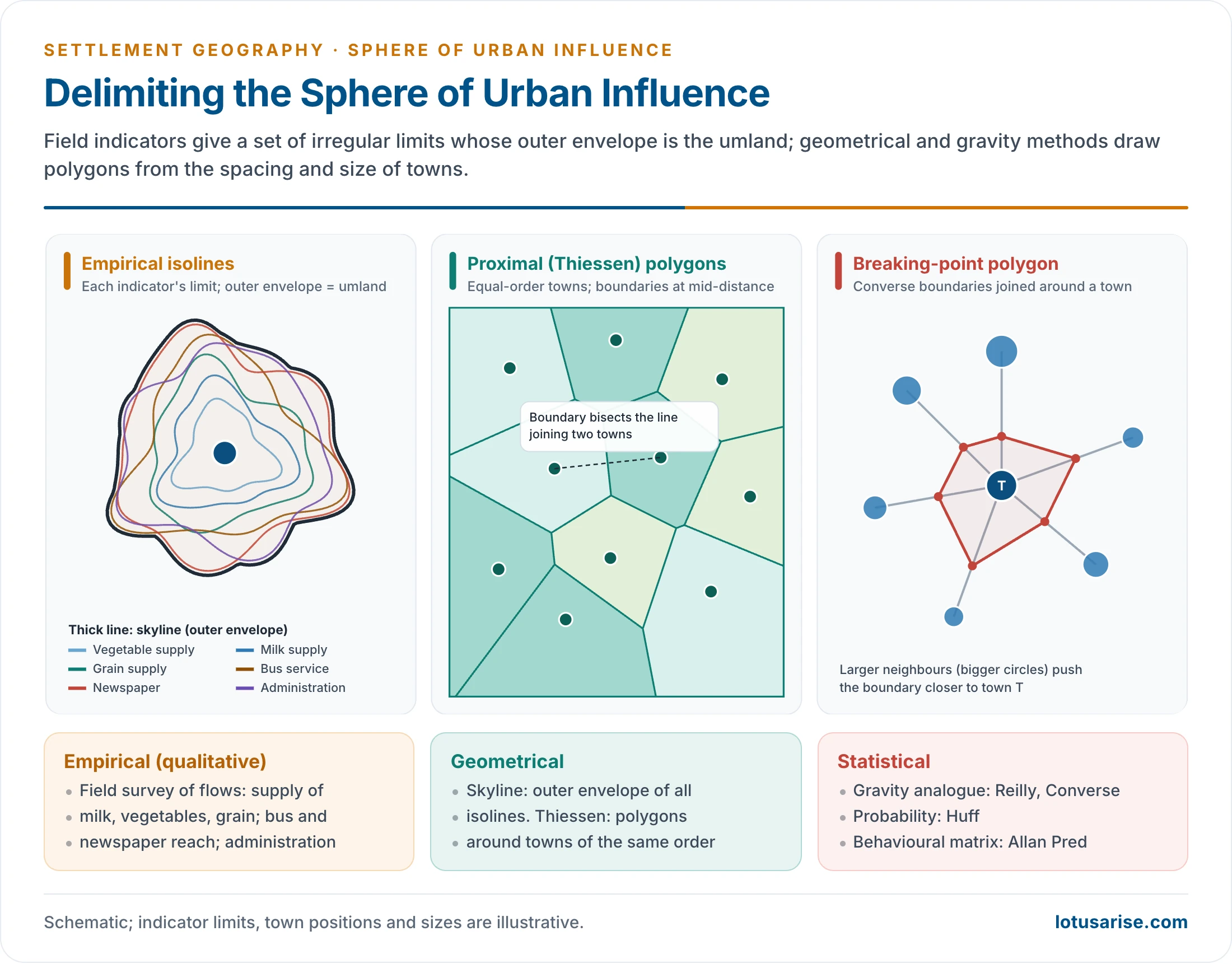
- Ram Lochan Singh’s study of Banaras (1955) was the first delimitation of the umland of an Indian city. He used two sets of criteria:
- Demand-based (inflow) variables: vegetable supply, milk supply and grain supply.
- He put the vegetable supply zone of the city at about 8 km.
- Supply-based (outflow) variables: bus services, newspaper distribution and administration.
- He mapped the radial limit of each good or service from the city centre and combined them.
- Demand-based (inflow) variables: vegetable supply, milk supply and grain supply.
- Similar studies followed for Allahabad (Ujagir Singh, 1961) and then the KAVAL towns (Kanpur, Allahabad, Varanasi, Agra, Lucknow; 1962).
- F. H. W. Green (1950) delimited urban hinterlands in England and Wales from the frequency of bus services.
- Steps in a field delimitation:
- choose indicators of inflow and outflow suited to the city’s size and functions;
- collect data for each village or ward: suppliers, commuters, newspaper agents, bus timetables, school and hospital registers;
- map the outer limit of each indicator as an isoline;
- combine the limits, by taking the outer envelope or the area where most indicators agree;
- check the result in the field and adjust it along roads and around barriers.
- Interaction indicators in common use:
- Newspaper circulation: a daily’s delivery limit marks where the city’s informational ties remain strong.
- Telephone connections: Christaller measured centrality from telephones as Z = Tz − Ez × (Tg / Eg), where Tz and Ez are the telephones and population of the place, and Tg and Eg those of the whole region. A positive surplus marks a centre serving others. Mobile-phone and transaction data now serve the same purpose.
- Commuting zone: the outer limit of daily journeys to work, the most functionally integrated part of the hinterland.
- Bus and rail service area: the city’s daily reach, useful for delimiting the urban fringe.
- The outer limit of city bus services is one of R. Ramachandran’s five criteria for the urban fringe around Indian cities.
- Milk and vegetable supply zones, the most perishable and so the shortest-range inflows.
- Retail trade areas, from customer surveys or vehicle registrations of shoppers. Grocery and luxury goods give different, nested trade areas.
- Hospital and school catchments: the areas from which patients and pupils come, used in health and education planning.
- Merits of empirical methods:
- they record actual flows, not assumed ones;
- they capture star-shaped and broken spheres along roads and across barriers;
- they suit Indian conditions, where official data are patchy but flows can be surveyed.
- Demerits:
- they are slow and costly, and depend on the observer’s choice of indicators;
- different indicators give different limits, so the final line involves judgement;
- the results date quickly as transport and markets change.
Quantitative Methods
Geometrical Methods
- Skyline method:
- The limit of each good or service is found from surveys and data and mapped up to its supply point.
- All the irregular polygons are superimposed. The outermost overlapping boundary is taken as the limit of the sphere.
- Proximal boundary method (Thiessen polygons):
- Towns of the same order are plotted on a map and each is joined to its neighbours.
- Perpendicular bisectors of these lines form irregular polygons, each taken as the sphere of one town.
- It assumes that people use the nearest centre.
- It ignores differences in size, so it works only for towns of the same order. Weighted polygons, which push the boundary towards the smaller town, correct for this.
- Skyline limits depend on the indicators chosen. A single far-reaching service, such as a newspaper, can inflate the sphere unless the envelope is checked against other indicators.
Statistical Methods
- Most quantification of the urban field rests on Newton’s law of gravitation, so these models are called gravity analogue models.
- Others are based on probability, and some on behavioural matrix analysis, which quantifies individual choices, demand and preferences from primary data.
- General gravity model: the interaction between two places is Iij = k × Pi × Pj / dij^b. Interaction rises with the product of their populations and falls with a power b of the distance between them. The same idea underlies the gravity model in geography, models of migration and traffic flows.
Reilly’s Law of Retail Gravitation
- William J. Reilly (1931) proposed the law to predict how two competing cities divide the trade of the area between them.
- Consumers are drawn to retail centres according to their size (mass) and the distance to be travelled.
- Two variables:
- Size: larger cities exert a stronger pull because they offer more variety, better quality and more specialised services.
- Distance: attraction falls with distance. Reilly used the inverse square of distance, so resistance rises steeply with distance.
- Trade-proportion formula: Bi / Bj = (Pi / Pj) × (dj / di)².
- B is the trade (or number of shoppers) a town k sends to city i or j; P is population; d is distance from k.
- Worked example: a town k of 1,000 people lies 12 km from city i (40,000) and 6 km from city j (5,000).
- Bi / Bj = (40,000 / 5,000) × (6 / 12)² = 8 × ¼ = 2 : 1.
- For every two people from k who go to i, one goes to j.
Converse’s Breaking-Point Formula
- Paul D. Converse (1949) rearranged Reilly’s law to find the breaking point: the point between two cities where their pull is equal and shoppers split their custom.
- Formula: dB = Dij / (1 + √(Pi / Pj)), where dB is the distance of the breaking point from the smaller town j, and Dij the distance between the two.
- Worked example: two cities 18 km apart have 45,000 and 5,000 people.
- dB = 18 / (1 + √9) = 18 / 4 = 4.5 km from the smaller town.
- Indian cases (Census 2011 UA populations, straight-line distances):
- Delhi (16.3 million) and Jaipur (3.0 million) are about 235 km apart. The breaking point lies about 71 km from Jaipur, far closer to the smaller city.
- Kanpur and Lucknow (2.92 and 2.90 million) are about 75 km apart. The breaking point falls almost at the midpoint, as near-equal cities share the area between them.
- Breaking points to all neighbouring cities, joined by straight lines, give a polygonal sphere with linear boundaries.
- The method gives a well-defined cut-off and is widely used in developed countries, but it is deterministic and often far from reality.
- Assumptions and their weaknesses:
- a uniform plain with equal transport in all directions;
- population as a sufficient measure of attraction, though two cities of equal size may differ greatly in shops, hospitals and colleges;
- similar consumers, all minimising distance;
- an exponent of 2 for distance, which in practice varies with the good, the region and the mode of travel.
Huff’s Probability Model
- David Huff (1963) treated the trade area as a probability surface. A consumer may use any of several centres, with a probability that rises with a centre’s attractiveness and falls with distance.
- Formula: Pij = (Sj / Tij^λ) ÷ Σ (Sk / Tik^λ), where S is the size of a centre, T the travel distance or time, and λ the friction of distance.
- Examples:
- If settlement k lies at the midpoint of two cities of equal size, the split is 50 : 50.
- If the distances are 18 km and 6 km for equal cities, with λ = 2, the split is 1 : 9.
- Unlike the breaking point, it yields overlapping trade areas and gradients rather than lines.
- It is widely used, with GIS, to choose sites for shopping centres, hospitals and bank branches. Its attraction measure can include floor space, variety or quality, not just population.

Behavioural Model
- Allan Pred (1967) proposed the behavioural matrix, which ranks decision-makers by the information they hold and their ability to use it.
- Behavioural models analyse individual decisions at a given time. They became very complex and could not fix the boundary of a city region precisely.
Limitations of Quantitative Methods
- Quantitative methods cannot precisely fix a city region because:
- primary data carry many discrepancies;
- people’s decisions change with time and circumstance;
- choices, tastes, emotions and values cannot be quantified;
- people are neither wholly economic nor wholly rational, so a law with rigid boundaries cannot capture their behaviour;
- results change with the measure of distance used: straight line, road distance or travel time, the last best reflecting congestion and service frequency.
- Star-shaped spheres: in many developing countries the sphere extends along roads and railways. Statistically drawn polygons then need modification.
- Areas that fail the statistical test but are functionally part of the sphere should be included, chosen by empirical criteria.
- The approach should be statistical cum empirical.
- The National Capital Region applied this approach: its delimited area projects outward along the main roads leaving Delhi.
- Developed countries differ: infrastructure runs in all directions, and growth along roadsides is weaker, partly through stricter environmental and land-use control.
- The city region is partly a mental construct. Demand, production and population keep changing, so qualitative methods often come closer to reality.
Multi-Criteria or Composite Methods
- The sphere has different extents for different functions, so the most complete approach uses several criteria together. It identifies the area where most indicators show the city’s dominance.
- Typical criteria: newspaper circulation, bus service limits, the commuting zone, retail catchments, hospital admissions and secondary-school attendance.
- The result is an irregular polygon, shaped by transport routes, physical barriers and competing centres.
- In India this approach informed the Calcutta Metropolitan District and the National Capital Region.
- The Calcutta Metropolitan Planning Organisation, set up in 1961, delimited the metropolitan district along both banks of the Hooghly for its Basic Development Plan (1966).
- The NCR combined commuting, built-up growth, transport links and administrative units, and was later enlarged by adding whole districts.
- GIS and remote sensing now combine census data, night-time lights, built-up maps, travel surveys and mobile-network data in such composite delimitation.
The Sphere of Urban Influence in the Indian Context
Census Units for the City and Its Spread
- The Census recognised that the city proper and its urban spread are not the same. Its units changed over time:
- Up to 1951: data only for individual towns.
- 1961: the town group, for neighbouring towns that function together.
- 1971: the urban agglomeration (UA): a continuous urban spread of a town and its outgrowths (railway colonies, university campuses, port areas), or two or more contiguous towns with their outgrowths.
- 1971–1991: the Standard Urban Area (SUA), a reporting unit for planning around towns of 50,000 or more. It included adjoining towns, outgrowths and rural pockets likely to urbanise. It was then discontinued.
- 1991 onward: towns and UAs. The Kolkata UA of 1991 had 129 urban units, such as Uluberia and Rishra, and 25 outgrowths, including the cantonments of Shyamnagar and Dum Dum.
- Outgrowths (OGs) are urban-like areas beside a statutory town, such as railway colonies, university campuses and port areas, counted with the UA though administered as villages.
- 2011: UAs remain the main unit. Million-plus UAs were Greater Mumbai (18.4 million), Delhi (16.3 million) and Kolkata (14.1 million) at the top.
Indian Examples
| City or region | Nature of sphere | Key features |
|---|---|---|
| National Capital Region | Statutory planned city region (NCR Planning Board Act, 1985) | NCT Delhi plus 14 districts of Haryana (Gurugram, Faridabad, Sonipat, Rohtak), 8 of Uttar Pradesh (Noida, Ghaziabad, Meerut, Hapur) and 2 of Rajasthan (Alwar); about 55,083 km²; 58.2 million people in 2011; counter-magnets beyond |
| Kolkata Metropolitan Area | Colonial port-industrial sphere | Along both banks of the Hooghly, including the old jute-mill belt; partition-era refugees widened the fringe |
| Mumbai Metropolitan Region | Western India’s dominant sphere | Mumbai, Thane, Navi Mumbai, Kalyan-Dombivli, Vasai-Virar; about 4,355 km² before its extension in 2019 to about 6,328 km² |
| Bengaluru Metropolitan Region | Sphere of the IT era | Electronic City, Whitefield and the Outer Ring Road; spread towards Devanahalli, Hosur and Tumakuru |
| Varanasi | Cultural and commercial sphere | National reach for pilgrimage; district-level reach for daily trade: overlapping spheres of different extent |
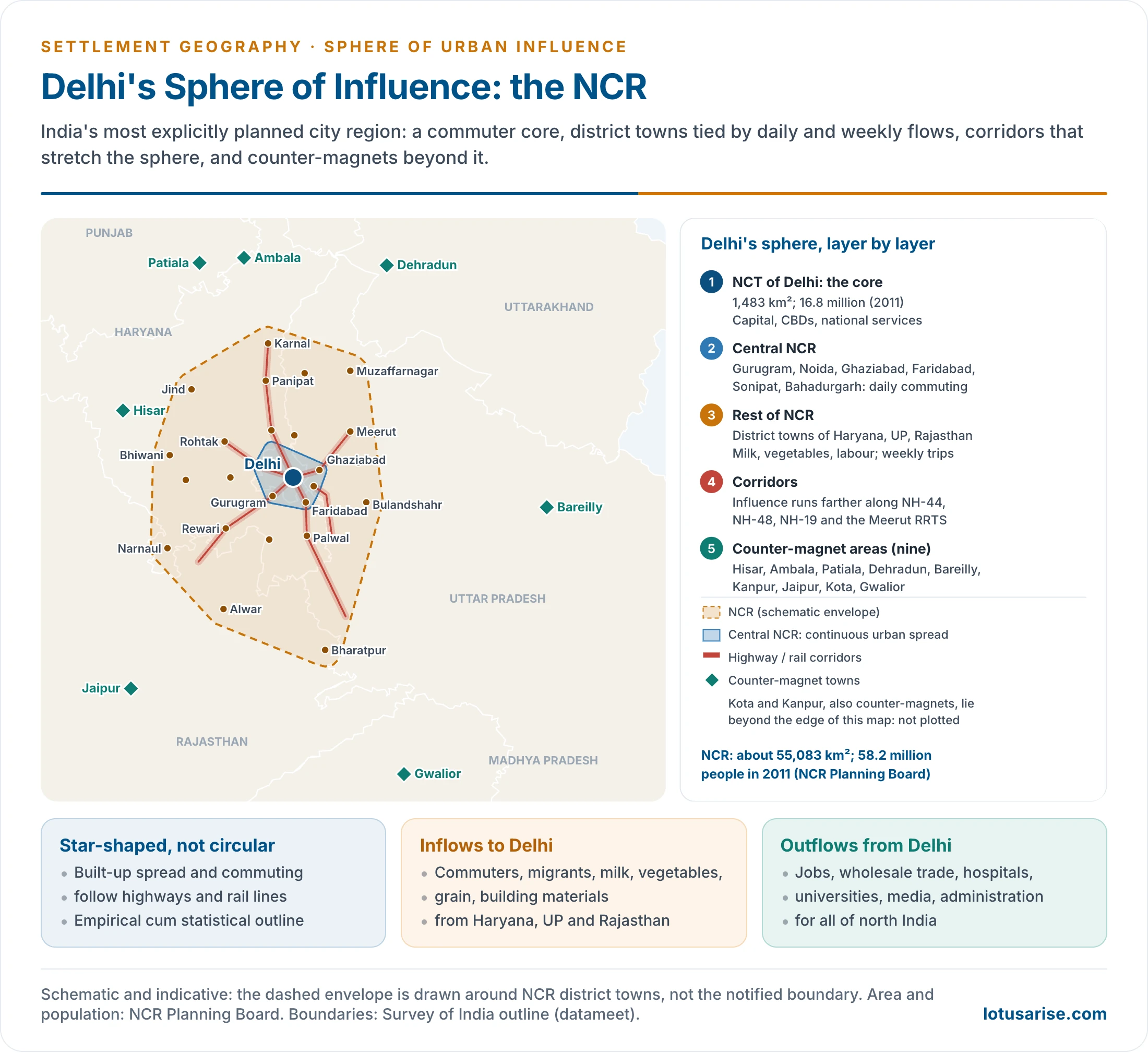
- Delhi’s sphere is India’s most explicitly planned one.
- The NCT is the core, ringed by the continuous urban spread of Central NCR (Gurugram, Noida, Ghaziabad, Faridabad, Sonipat, Bahadurgarh).
- District towns supply milk, vegetables, labour and building materials.
- Influence stretches along NH-44, NH-48, NH-19 and the Delhi–Meerut Namo Bharat (RRTS) line.
- Nine counter-magnet areas lie beyond (Hisar, Ambala, Patiala, Dehradun, Bareilly, Kanpur, Jaipur, Kota, Gwalior), meant to intercept migrants and grow as regional centres. The first five chosen, under Regional Plan 2001, were Hisar, Gwalior, Patiala, Kota and Bareilly.
- Other metropolitan spheres:
- Kolkata: the sphere follows the Hooghly in a linear belt of twin-bank towns, with a regional reach over West Bengal, Bihar, Jharkhand, Odisha and the North-East through port, rail and wholesale trade.
- Mumbai: the financial capital’s daily sphere extends north to Vasai-Virar and Palghar and south-east to Navi Mumbai, Panvel and the Pune corridor; its business sphere is national.
- Bengaluru and Hyderabad: IT-led growth has pushed their spheres along ring roads and airport corridors, drawing skilled migrants from across the south and beyond.
- Chennai: port, automobile and electronics industries extend its sphere along the Sriperumbudur and Gummidipoondi corridors.
- Varanasi: a city of several spheres at once. Its pilgrimage and cultural sphere is national, its silk-weaving and handicraft trade reaches distant markets, and its daily commercial sphere covers only the surrounding districts.
- Institutions: the 74th Constitutional Amendment (1992) provides for Metropolitan Planning Committees for areas of 10 lakh or more, the constitutional recognition that planning must follow the city’s sphere. Metropolitan development authorities (MMRDA, KMDA, BMRDA) perform the role in practice.
- In June 2026 the NCR Planning Board decided to retain the NCR’s present extent under the Regional Plan 2041, and to develop transit-oriented “Namo Cities” at stations on the RRTS lines.
Why Western Models Apply Imperfectly to India
- Topographic diversity: mountains, deserts, deltas and plateaus break the isotropic plain that Christaller and Reilly assume.
- Socio-economic inequality: richer groups bypass lower-order centres; poorer groups depend on local services. Consumer behaviour is not uniform.
- Multipurpose trips: consumers combine several purchases and services in one trip to a higher-order centre, rather than visiting the nearest centre for each.
- Cultural and religious factors: pilgrimage towns, temple towns and dargah economies have non-market spheres that the models do not capture.
- Colonial legacy: Mumbai, Kolkata and Chennai acquired spheres by administrative and commercial design, distorting the hierarchy for good.
- Rapid unplanned urbanisation: urban sprawl and fringe growth run ahead of infrastructure, so boundaries are unstable.
- Periodic markets (haats) carry rural exchange alongside fixed central places.
Primate Cities and Their Spheres
- In many developing countries a primate city makes the whole nation its sphere: Bangkok, Lima, Dhaka, Manila, Nairobi.
- Smaller cities keep only truncated, low-order spheres in its shadow.
- Their highest-order functions (ministries, head offices, universities, specialist hospitals) are concentrated in the capital.
- India has no national primate city. Each metropolis dominates a regional sphere: Delhi the north-west, Kolkata the east, Mumbai the west, Chennai, Bengaluru and Hyderabad the south.
- Most State capitals dominate their States’ spheres.
- Evaluation: primate dominance concentrates scarce high-order services efficiently, but it also drains capital and talent from smaller towns and leaves large left-out areas. Strengthening secondary cities spreads the spheres of high-order services more evenly.
Changing Spheres in a Global and Digital Age
- Global cities such as London, New York and Tokyo have spheres of finance, media and corporate control that are worldwide. Their links with one another can be stronger than their links with their own hinterlands.
- Indian metros are part of these networks: Mumbai for finance, Bengaluru and Hyderabad for software and global capability centres.
- Digital services blur boundaries. A village customer may buy from a metropolitan e-commerce warehouse or consult a city doctor online, so spheres become networks of flows rather than contiguous areas.
- The physical sphere still matters for daily goods, commuting, perishables and in-person services, so the classical delimitation methods remain relevant.
Planning Implications
- The sphere of influence has direct planning value. Urban planning cannot stop at the municipal boundary, because migration, commuting, land-use change and infrastructure demand all operate at the scale of the sphere.
- Metropolitan planning regions:
- The logical planning unit is the whole sphere, not the municipal city.
- India’s NCR, the Mumbai Metropolitan Region and the Bengaluru Metropolitan Region are defined at this scale.
- Decisions on land use, transport, housing and industry are taken at the regional level.
- Green belts:
- Agricultural or open land around a city is protected to control sprawl.
- Ebenezer Howard (1898) first visualised the idea. A green belt was proposed around London in 1935 and given legal backing in 1938.
- Delhi’s Master Plan provides a green belt, though enforcement has been weak.
- Counter-magnets and satellite towns:
- When a sphere becomes over-extended, planners develop counter-magnets and new towns to draw investment and people away from the core.
- Examples: Navi Mumbai for Mumbai; Noida and Gurugram for Delhi; and the NCR’s counter-magnet towns.
- New towns:
- The idea arose in England at the end of the 19th century and was implemented after the Second World War to receive overflow population from London.
- India’s new towns (Chandigarh, Gandhinagar, Naya Raipur) follow the concept.
- Smart Cities Mission (2015–2025): 100 cities prepared area-based and pan-city plans, strengthening secondary cities in the hierarchy.
- PM Gati Shakti (2021) and rapid rail and expressways extend the effective commuting zone of large cities. Greater connectivity means a larger, more integrated sphere.
- Conclusion: no city exists in isolation. The sphere of influence is the spatial fingerprint of a city’s relations with its region, and managing it through regional plans, green belts, counter-magnets and connectivity is central to the quality of urban life in India.
Previous Year Questions
1986Define the urban sphere of influences and discuss different methods of determining the spheres of influence of cities.1993Define Umland and discuss, with specific examples, the criteria for its delimitation.1998Discuss the concept of city region and referring to Indian cities, examine critically functional indicators used for delimiting the city region.2003Examine the concept of sphere of urban influence and discuss the qualitative and quantitative methods used in its delimitation.2012Write short note on Relevance of distance decay principle in Indian cities.2013City-regions as territorial unit for regional planning and development.2014Explain the qualitative and quantitative methods of delineation of the sphere of urban influence.2025Critically evaluate the role of primate cities in dominating the urban spheres of influence in developing countries.





Well curated article.Thank you
May I know the sources, as whole aspect is not covered in Majid Husain
Sources could be rushikesh sir notes then you can also prefer internet….nd may go through topper copies
From which website you get the toppers copies
Visit: https://lotusarise.com/optional/geography-optional-toppers-answer-copy/
thanks a lot sir
This is really a good content.