- The gravity model predicts spatial interaction: the flow of people, goods, money or messages between places. Flow rises with the size of the places and falls with the distance between them.
- It is an analogue model borrowed from Newton’s law of gravitation, and one of the most widely used models of flows in the social sciences.
- It gives one logic to several fields: migration, retail trade areas, international trade, transport planning and the delimitation of functional regions.
The Model

The Newtonian Analogy
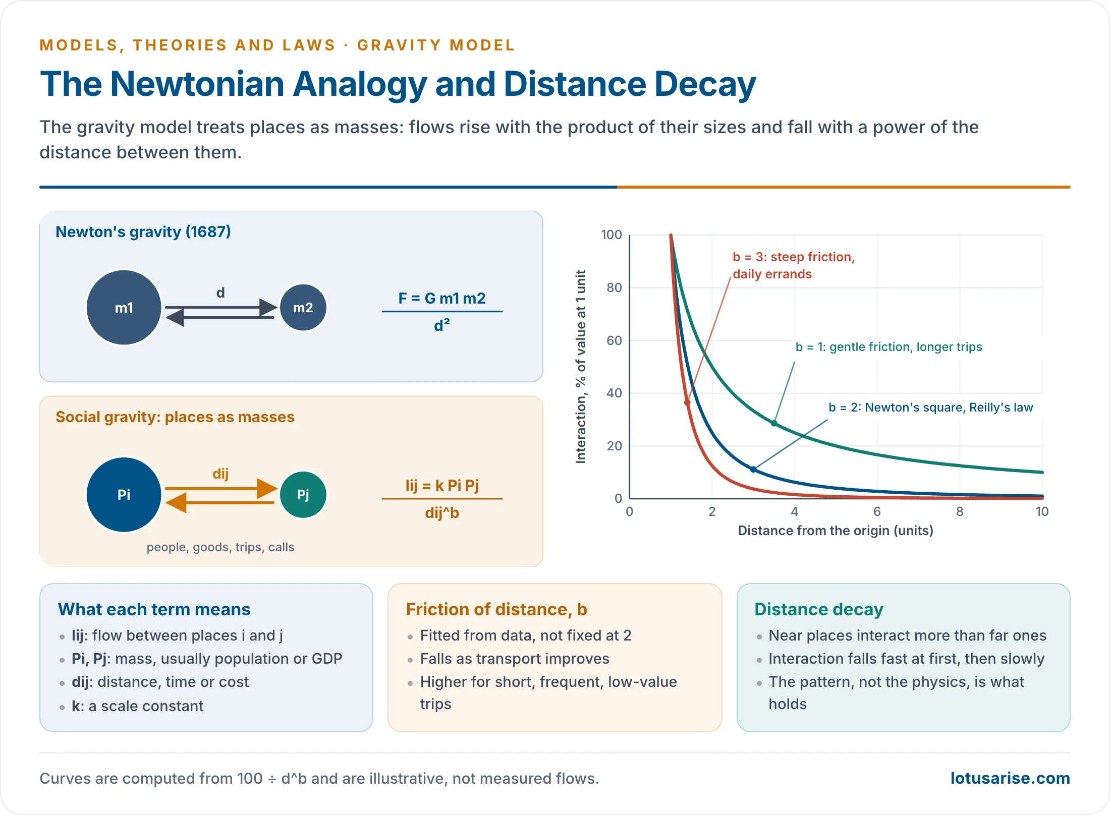
- Newton (1687): F = G × m1 × m2 ÷ d². Attraction varies with the product of two masses and inversely with the square of the distance.
- Gravity model: Iij = k × Pi × Pj ÷ dij^b
| Symbol | Stands for | Explanation |
|---|---|---|
| Iij | Interaction | Trips, migrants, trade or calls between i and j |
| Pi, Pj | Mass | Population, GDP, jobs or floor space |
| dij | Distance | Kilometres, travel time or cost |
| b | Friction of distance | Fitted from data; not fixed at Newton’s 2 |
| k | Constant | Scales the result to the flow measured |
- Distance decay lies at the core: nearer places interact more, and the fall is steep at first and then gentle.
- The exponent b is high for short, frequent, low-value trips and falls as transport improves.
- Distance stands for a bundle of frictions: cost, time, poor information, cultural difference and legal barriers.
- A quick test (illustrative): take two places whose populations multiply to give a flow of 100 at some distance. Doubling the distance cuts the flow to 50 if b = 1 and to 25 if b = 2, while doubling one population doubles it. This is why a good estimate of b matters more than the formula.
How the Model Developed
| Scholar, year | Contribution |
|---|---|
| Henri-Guillaume Desart, 1846 | Belgian engineer; early empirical form from railway passenger data |
| Henry Charles Carey, 1858 | Principles of Social Science: people gravitate to each other as matter does; first statement in social science |
| Ernst Georg Ravenstein, 1885 | Migration currents grow with the centre’s absorbing power and weaken with distance |
| William J. Reilly, 1929, 1931 | The Law of Retail Gravitation: trade drawn by two cities from the area between them |
| John Q. Stewart, 1940s | Astronomer at Princeton; “demographic gravitation” and population potential |
| George Kingsley Zipf, 1946 | P1P2/D hypothesis for intercity movement; least effort as the reason |
| Paul D. Converse, 1949 | Breaking point between two cities |
| Jan Tinbergen, 1962 | Shaping the World Economy: gravity equation for trade |
| David L. Huff, 1963 | Probabilistic trade areas |
| Alan G. Wilson, 1967, 1970 | Derived spatial interaction from entropy, without the physics analogy |
| James E. Anderson, 1979 | Economic foundation for the trade equation |
- Wilson’s family comes in four forms: unconstrained, production-constrained, attraction-constrained and doubly constrained. Each fixes known totals at origins, destinations or both, and the fitted flows must add up to them.
- Geographers met these ideas through social physics and the locational school, which made distance decay a basic element of movement.
Stewart’s Population Potential
- Stewart moved from a pair of places to a whole field. Population potential at i is the sum of all populations, each divided by its distance from i:
- Vi = Σ (Pj ÷ dij)
- It measures how close a place is to people in general, and maps show a smooth surface peaking at the great urban cores.
- Chauncy D. Harris (1954) applied the same form to market potential to explain industrial location, and Walter G. Hansen (1959) used it for accessibility in land-use planning.
Reilly’s Law and the Breaking Point
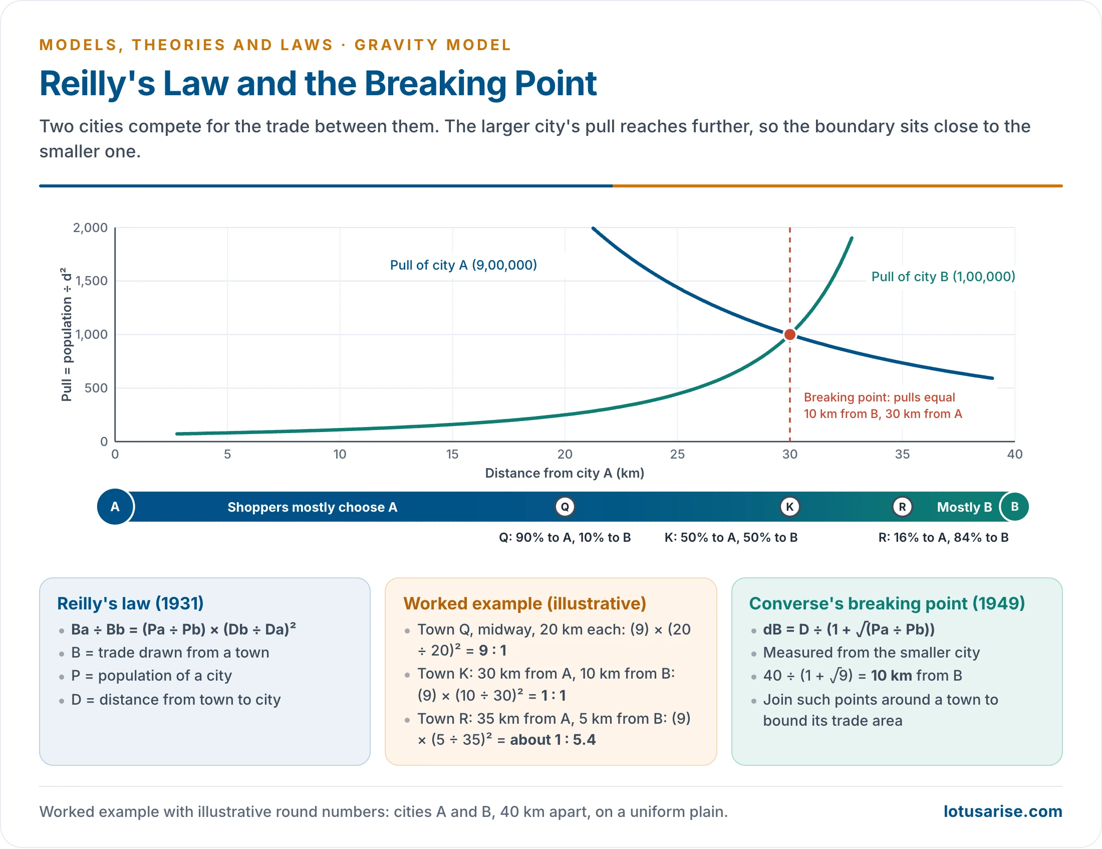
- Reilly’s law of retail gravitation: two cities draw trade from a town between them in direct proportion to their populations and in inverse proportion to the square of their distances from it.
- Ba ÷ Bb = (Pa ÷ Pb) × (Db ÷ Da)²
- Reilly found the population exponent to be about 1 and the distance exponent to lie between 1.5 and 2.5, using 2 as the working value.
- Converse’s breaking point finds where the two pulls are equal, measured from the smaller city:
- dB = D ÷ (1 + √(Pa ÷ Pb))
- Breaking points with all neighbours, when joined, bound a town’s trade area.
- Worked example (illustrative): cities A (9,00,000) and B (1,00,000) are 40 km apart, so Pa ÷ Pb = 9.
- Breaking point: 40 ÷ (1 + √9) = 10 km from B, 30 km from A.
- Town Q, midway at 20 km from each: 9 × (20 ÷ 20)² = 9 : 1 in favour of A.
- Town K, at the breaking point: 9 × (10 ÷ 30)² = 1 : 1.
- Town R, 35 km from A and 5 km from B: 9 × (5 ÷ 35)² = 9 ÷ 49, or about 1 : 5.4 in favour of B.
- The larger city’s field reaches further. That is why the boundary sits near the smaller city, as with the Delhi–Jaipur case in spheres of urban influence.
Huff’s Probability Model
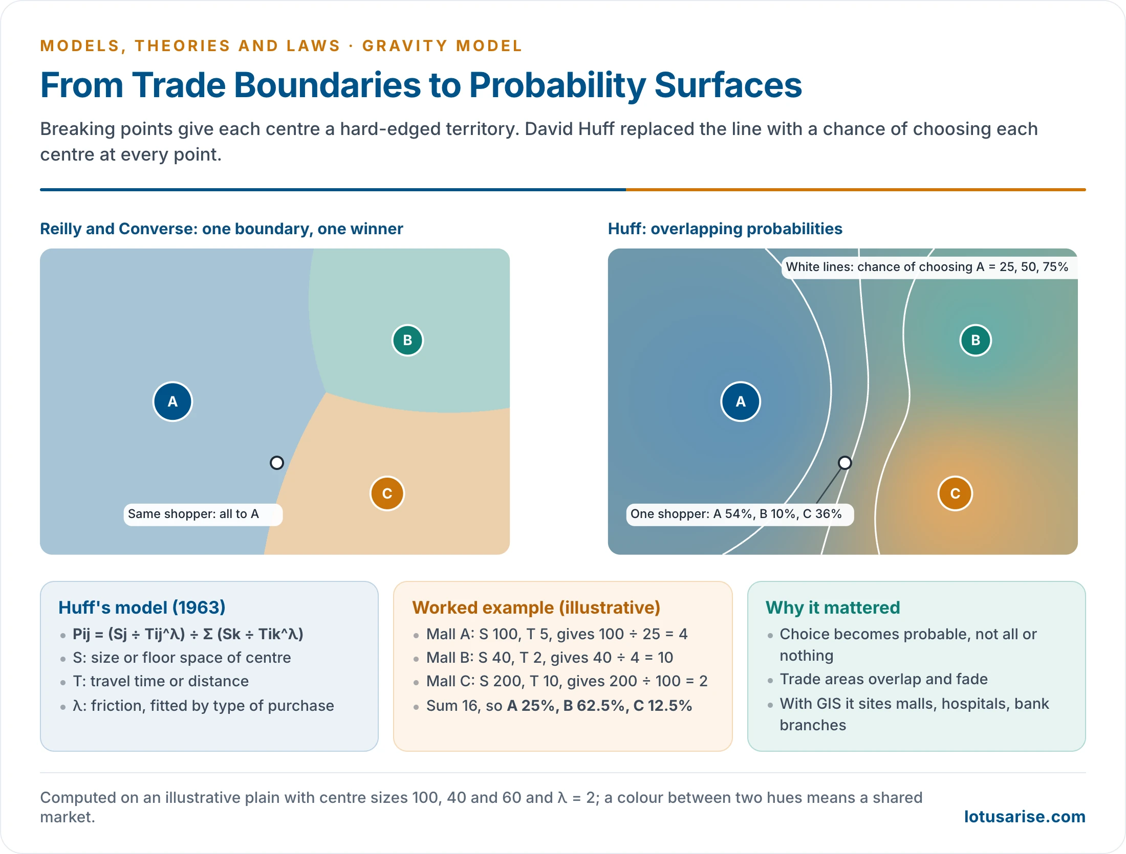
- David L. Huff (1963) replaced the line with a probability surface. A shopper can go anywhere, with a chance that depends on every centre on offer:
- Pij = (Sj ÷ Tij^λ) ÷ Σ (Sk ÷ Tik^λ)
- S is the size or floor space of a centre, T travel time or distance, and λ the friction, fitted by type of purchase.
- Worked example (illustrative, λ = 2):
- Mall A: size 100, 5 minutes away: 100 ÷ 25 = 4.
- Mall B: size 40, 2 minutes: 40 ÷ 4 = 10.
- Mall C: size 200, 10 minutes: 200 ÷ 100 = 2.
- The sum is 16, so the chances are A 25%, B 62.5%, C 12.5%.
- What changed:
- Trade areas now overlap and fade.
- The model begins from individual choice rather than from aggregates.
- Attraction became floor space and variety, not population.
- With GIS it now sites shopping centres, hospitals and bank branches.
Applications
Migration
- Zipf’s form: migrants between two places vary with P1P2/D. The theories of migration treat this alongside Ravenstein and Samuel A. Stouffer’s intervening opportunities (1940), which replace distance with the opportunities passed on the way.
- Economic Survey 2016–17 fitted a gravity equation to Indian unreserved railway passenger flows:
- A 1% rise in distance cut net flows between States by about 1.66%, roughly twice the effect on goods: people flow less easily than goods.
- States sharing a border saw about 65% more migration, and flows within a State were about four times those across State lines.
- Language was not a significant barrier within India, unlike across countries.
- Economic Advisory Council to the Prime Minister (2024), using railway ticketing and mobile roaming data, found patterns in line with gravity models, with short-distance moves the largest share.
Trade
- Tinbergen (1962) made it the workhorse of international trade: exports rise with the two economies’ GDP and fall with distance.
- The distance effect has not died. Reviewing 1,467 estimates in 103 papers, Anne-Célia Disdier and Keith Head (2008) found a mean elasticity of about 0.9: 10% more distance means about 9% less trade. It rose after mid-century, despite cheaper transport.
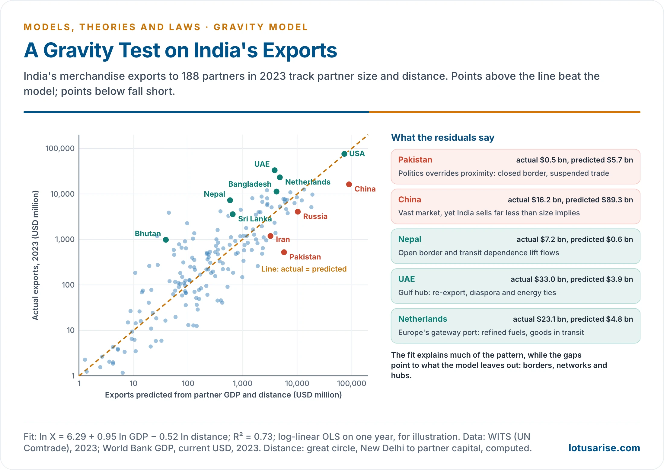
- India’s own exports fit the pattern. A simple fit for 188 partners in 2023 gives exports rising with partner GDP (elasticity 0.95) and falling with distance (elasticity 0.52), explaining about 73% of the variation in log terms.
- The USA sits almost on the prediction.
- Pakistan takes about a tenth of what its size and nearness imply, since politics overrides proximity. China takes about a fifth.
- Nepal, Bhutan, the UAE and the Netherlands exceed it, through open borders, transit dependence, diaspora and hub roles.
Retail and Services
- Reilly, Converse and Huff delimit trade areas. Real spheres of influence in India bend along roads and around rival towns, away from the neat breaking points.
- Similar logic sets catchments for hospitals, colleges and banks. Stewart’s early work measured the drawing power of a college on its undergraduates.
Transport
- Trip distribution is the second stage of the four-stage travel demand model: trip generation, distribution, mode choice, assignment. Trips between zones follow size and travel cost.
- The NCR Planning Board’s transport model used a gravity model for trip distribution, validated against trip-length distribution and mean trip length. Comprehensive Mobility Plans for Indian cities use the same four-stage structure.
Regionalisation
- Gravity estimates can stand in for missing flow data when functional regions are delimited, as a second-best to observed flows.
Critique
Limitations
| Issue | Problem | Later response |
|---|---|---|
| Physics analogy | Places are not masses; early versions had no behavioural reason | Zipf’s least effort, Huff’s choice, Wilson’s entropy, Anderson’s economics |
| Mass | Population hides income, jobs and specialisation | GDP, floor space, vacancies |
| Distance | Straight lines ignore roads, rivers and time | Network time, generalised cost |
| Exponent | b differs by place, date, mode and good, so results do not transfer | Fresh calibration for each case |
| Intervening places | A pair ignores what lies between or around | Stouffer; Anderson and van Wincoop’s “multilateral resistance” (2003) |
| Barriers | Borders, language, visas and war are left out | Added variables for border and language |
| Aggregate | Individual motive is hidden | Discrete choice, agent-based models |
| Static | A snapshot, with no change through time | Dynamic models, panel data |
| Estimation | Logs drop zero flows and bias results | Poisson method of João Santos Silva and Silvana Tenreyro (2006) |
- Description, not explanation. It says how much, not why, and is silent on who gains. Behavioural and radical geographers object on that ground.
- Isotropic surface: Reilly assumes a uniform plain and identical consumers, while real shoppers differ by income, gender and social group as well as distance.
- Digital connectivity weakens some frictions. Yet distance effects persist even for online goods, because trust, information and networks remain local.
Current View
- Its central regularity has lasted better than most in human geography, and it fits with Waldo Tobler’s first law (1970), which holds that near things are more related than distant ones.
- Its best use is as a benchmark. Where flows depart from the prediction, as with Pakistan or the Gulf, the gap itself is the geography to be explained.
Previous Year Questions
2016Discuss the application of Gravity model in Geographical studies.1999Write short note: Gravity model.