

- Migration is one of the three components of population change, with fertility and mortality. It is the most volatile of the three and the most sensitive to policy, and it can change the size and make-up of a population abruptly.
- Unlike births and deaths, migration is selective by age, sex and skill. It reshapes both the place left behind and the place of arrival.
- Male-selective out-migration from rural areas leads to the feminisation of agriculture, lower fertility at the origin and a higher dependency ratio.
- No single theory explains migration. Explanations have moved from empirical laws in the late 19th century to behavioural, economic, structural and network theories, each working at a different scale.
Concept and Nature of Migration

Definition
- The United Nations (Multilingual Demographic Dictionary, 1958) defines migration as spatial mobility between one geographical unit and another, involving a permanent or semi-permanent change of usual residence.
- Migration therefore combines a move across space, a time threshold and a change in residence status.
- Censuses and surveys fix the threshold: six months of stay in India’s PLFS, 12 months for international migrants in UN statistics.
- Mobility is the wider term. It includes moves that do not change usual residence:
- Commuting: daily movement between home and work.
- Circulation: short-term, repetitive or cyclical moves, such as seasonal labour and transferable jobs.
- Transhumance: seasonal vertical movement of herders with their flocks, for example the Gaddis of Himachal Pradesh and the Bakarwals of Jammu and Kashmir.
- Refugees and other forced migrants cross borders under compulsion. Earlier demographic definitions left them out; migration studies now treat them as a distinct category, defined in international law.
| Basis | Mobility | Migration |
|---|---|---|
| Scope | All movement of people | A subset of mobility |
| Residence | Usual residence may not change | Usual residence changes |
| Time | Hours to months, often repeated | Beyond a threshold (6 or 12 months) |
| Examples | Commuting, seasonal circulation, pilgrimage | Rural–urban move, marriage migration, emigration |
Demographic Significance
- Size: migration adds to or subtracts from natural increase. In many developed countries it now outweighs natural increase as the source of growth.
- Structure: because movers are mostly young adults, in-migration lowers the median age at the destination and out-migration ages the origin.
- The Gulf states have a huge male bulge at working ages; the hill districts of Uttarakhand have a deficit of young men.
- Composition: migration changes the ethnic, linguistic and religious mix of places and spreads ideas, skills and fertility norms.
Why Many Theories?
- Migration is multi-causal:
- Economic: jobs and wages.
- Social: education, marriage, family.
- Political: conflict and state policy.
- Environmental: disasters and climate change.
- It is also shaped by perception and aspiration. Two people in the same village facing the same conditions can decide differently.
- Theories therefore come from several disciplines (geography, economics, sociology, political science) and work at three levels:
- Micro: the individual decision-maker.
- Meso: households, networks and institutions.
- Macro: regional and global structures.
| Level | Unit of analysis | Core question | Main theories |
|---|---|---|---|
| Micro | Individual | Why does this person move? | Lee’s push–pull, Sjaastad’s human capital, Todaro, behavioural models |
| Meso | Household, network, institution | How do moves continue and cluster? | NELM, network theory, cumulative causation, migration systems, institutional theory |
| Macro | Region, nation, world economy | Where and why do flows arise? | Ravenstein, gravity, Zelinsky, Lewis, neoclassical macro, dual labour market, world systems |
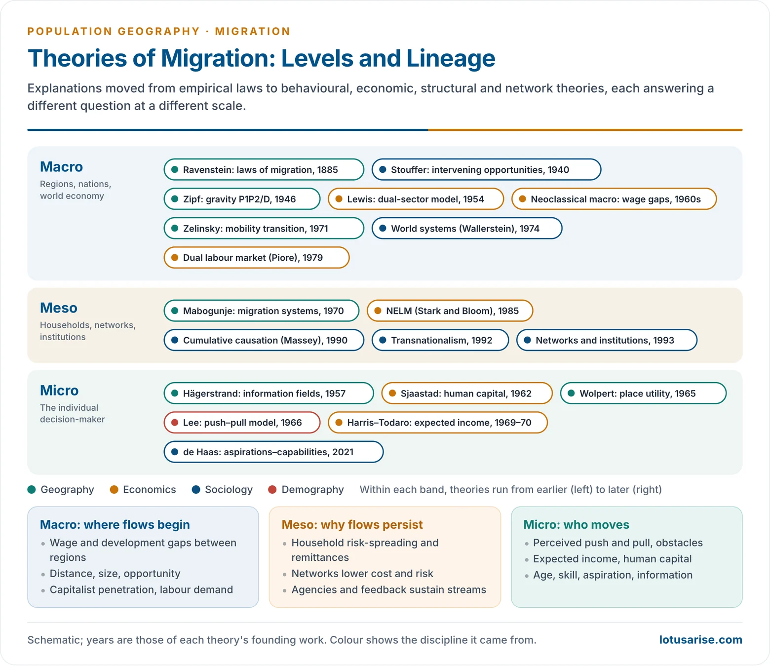
- Evolution in brief:
- Late 19th century: empirical generalisations from census data (Ravenstein) and a positivist tradition.
- Early 20th century: migration seen as a response to population pressure on resources, in the line of Thomas Robert Malthus (1798).
- 1940s–1960s: spatial interaction models (gravity, intervening opportunities) and the behavioural turn (Lee).
- 1950s–1970s: neoclassical and dual-economy models of rural–urban migration (Lewis, Sjaastad, Todaro).
- 1970s–1980s: structural views (dual labour market, world systems) and household strategies (NELM).
- 1990s onward: networks, cumulative causation and transnationalism, and new themes such as climate-linked migration, the feminisation of migration, and student and digital-skill mobility.
Spatial and Behavioural Models
Ravenstein’s Laws of Migration (1885, 1889)
- Ernest George Ravenstein, a German-born geographer working in London, read the birthplace data of the 1871 and 1881 British censuses. He presented his “Laws of Migration” in 1885 and 1889, the first systematic generalisation about migration.
- His central idea was absorption and dispersion:
- Counties of absorption had more residents than people born there: they received migrants.
- Counties of dispersion had fewer residents than people born there: they sent migrants out.
- People flow from less favourable to more favourable areas, that is, from dispersion to absorption.
- His main generalisations:
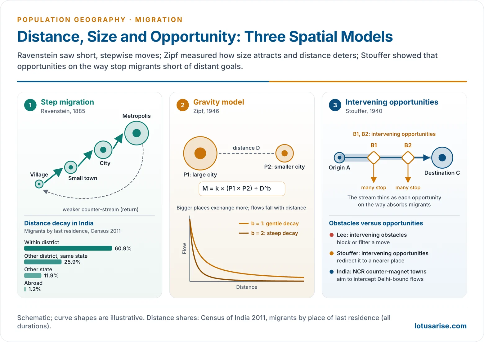
- Most migrants go short distances, and numbers fall with distance (distance decay).
- Migration proceeds step by step: village to town to city.
- Long-distance migrants head for great centres of commerce and industry.
- Each stream produces a weaker counter-stream.
- Town natives are less migratory than rural people.
- Women dominate short-distance moves and men long-distance ones.
- Economic motives are the main cause, and migration increases as industry, commerce and transport develop.
- The laws are empirical, not a theory of decision. They say little about why individuals move, and they were drawn from one industrialising country. Later geographers turned them into distance-decay and gravity formulations.
Gravity Model and Zipf’s P1P2/D Hypothesis (1946)
- The gravity analogy in social science goes back to Henry Charles Carey (1858) and Ravenstein. George Kingsley Zipf (1946) gave it a migration form in his P1P2/D hypothesis:
- Migration between two places is directly proportional to the product of their populations and inversely proportional to the distance between them.
- Migration between places i and j = k × (Pi × Pj) ÷ Dij^b, where the distance exponent b is fitted from data. It is usually between 1 and 2, not fixed at Newton’s 2.
- Zipf grounded it in his principle of least effort: people prefer shorter, easier moves.
- William J. Reilly (1931) used the same logic for retail trade areas (the law of retail gravitation), not migration.
- Distance in these models stands for a bundle of frictions:
- cost of travel and relocation;
- visas and immigration rules;
- language and cultural difference;
- poorer information about distant places.
- West Africa shows distance and friction at work. Most West African migrants go to neighbouring countries (Côte d’Ivoire, Nigeria, Ghana) within the ECOWAS free-movement zone; far fewer reach Europe, where cost and visa barriers are high.
- Indian evidence:
- Large origins and large destinations generate the biggest flows: Uttar Pradesh and Bihar to Delhi and Maharashtra.
- About 61% of migrants by last residence in Census 2011 had moved within their own district.
- A 2024 study for the Economic Advisory Council to the Prime Minister, using railway ticketing and mobile-roaming data, found flows in line with gravity models: short-distance moves form the largest share, and districts around Delhi, Mumbai, Kolkata, Chennai and Bengaluru are the main origins.
- Strengths:
- Simple and measurable. It predicts the volume of flows well at the internal scale.
- It is the basis of later spatial interaction and transport models.
- Limitations:
- It says how much, not why: it ignores push–pull causes, policies and networks.
- It cannot handle step migration or intervening opportunities.
- Cheap transport and digital connectivity have weakened the pull of physical distance. Long-distance flows such as India to the Gulf and the USA are shaped more by networks and visa regimes than by kilometres.
- Later refinements replace raw population with income, unemployment or job vacancies, and add dummy variables for shared language or colonial ties.
Stouffer’s Intervening Opportunities (1940)
- Samuel A. Stouffer (1940) argued that opportunities, not distance as such, govern migration:
- The number of people going a given distance is directly proportional to the opportunities at that distance and inversely proportional to the intervening opportunities between origin and destination.
- Migrants tend to stop at the nearest place that meets their need.
- Intervening opportunities are jobs, land, schools or safety met on the way. They redirect flows, unlike Lee’s intervening obstacles, which block or filter them.
- In 1960 Stouffer added competing migrants: flows also fall when many others compete for the same opportunities at the destination.
- Examples:
- A student who gets into an IIT or AIIMS has no need to go abroad: the domestic seat is an intervening opportunity.
- NCR planning uses the idea. Gurugram, Noida and Ghaziabad, and counter-magnet towns such as Hisar, Kota, Bareilly and Gwalior, are meant to intercept migrants bound for Delhi.
- In southern Africa, migrants from Zimbabwe and Mozambique stop in South Africa, the region’s economic core, rather than attempting Europe.
- Evaluation:
- More realistic than pure distance models. It explains why migrants stop short of distant goals, and it suits urban and regional planning.
- “Opportunities” are hard to measure objectively. The model ignores networks, culture and policy, and cannot explain long jumps driven by a strong pull, such as Kerala to the Gulf.
| Model | Key variable | Prediction | Main gap |
|---|---|---|---|
| Ravenstein (1885) | Distance, economic pull | Short, stepwise moves to industrial centres | Descriptive, not explanatory |
| Zipf / gravity (1946) | Population size, distance | Flow ∝ (Pi × Pj) ÷ D | Ignores causes and policy |
| Stouffer (1940) | Opportunities in between | Migrants stop at the nearest adequate place | Opportunities hard to measure |
| Lee (1966) | Perceived factors, obstacles | Volume and selectivity depend on perception | Hard to quantify perception |
Lee’s Theory of Migration (1966)
Core Idea
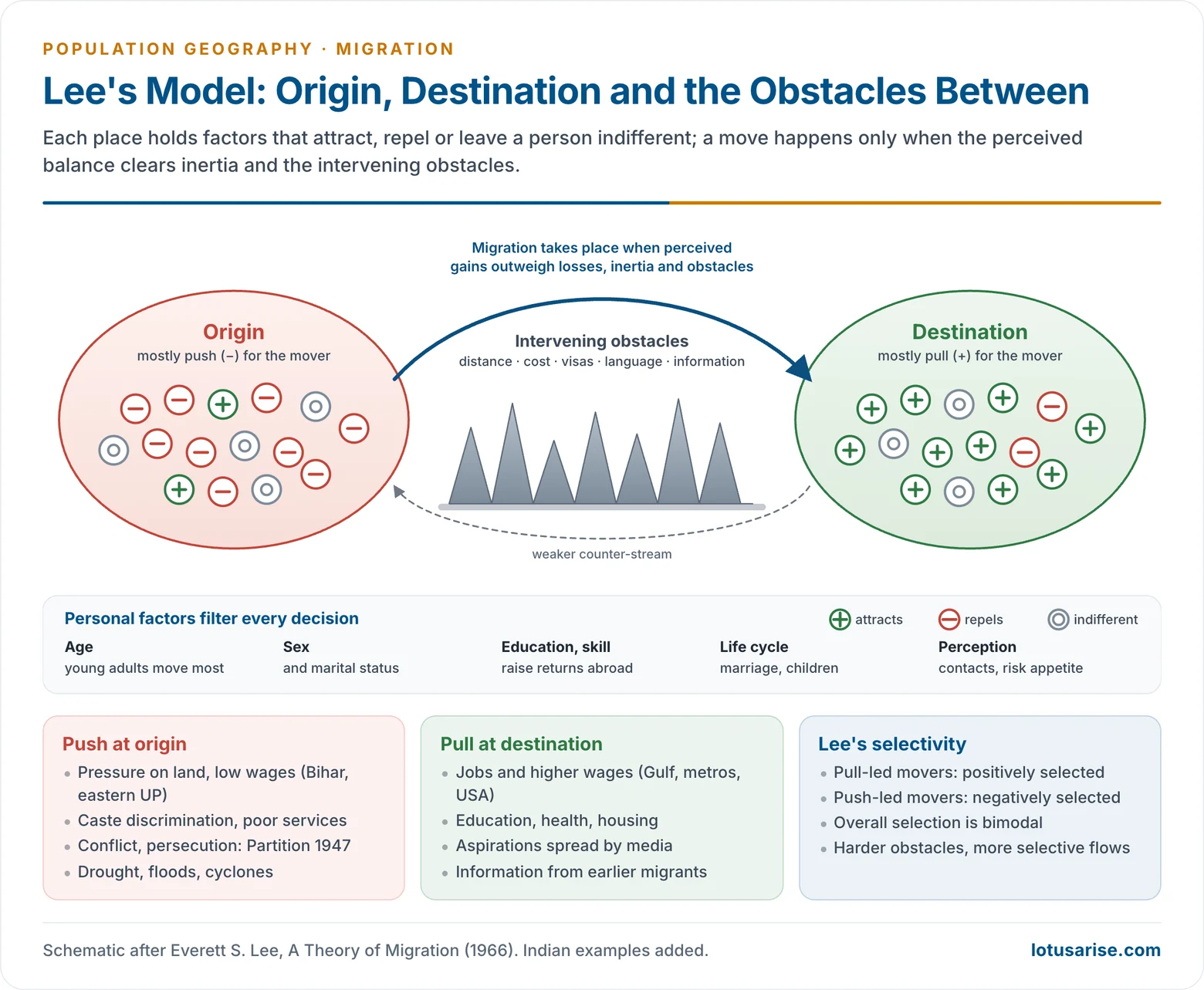
- Everett S. Lee (1966) recast Ravenstein’s laws as a behavioural model of decision-making.
- Every move involves four sets of factors:
- Factors at the origin (mainly push).
- Factors at the destination (mainly pull).
- Intervening obstacles between the two.
- Personal factors of the migrant.
- At both origin and destination, each factor can be positive (+), negative (−) or neutral (0) for a given person.
- Good schools are a plus for a family with children and neutral for a childless person.
- People know their origin intimately but the destination only through imperfect information, so an element of uncertainty always remains.
- A move takes place only when the balance of perceived pluses and minuses is strong enough to overcome natural inertia and the obstacles.
- Migration is therefore subjective and selective, not an automatic reaction to wage gaps.
The Four Sets of Factors
- Push factors (origin):
- Population pressure on land: small holdings, unemployment, low wages (eastern Uttar Pradesh, Bihar).
- Economic backwardness: few jobs outside farming, little industry.
- Social factors: caste discrimination, poor schools and health care.
- Political factors: war, partition, persecution (the Partition of 1947, the Kashmiri Pandit exodus of 1990, Palestinian displacement).
- Environmental stress: drought, floods, cyclones.
- Pull factors (destination):
- Jobs and higher wages, the strongest pull (the Gulf, the USA, Indian metros).
- Services: education, health care, housing, transport.
- Aspirations and lifestyle, spread through media and education.
- Information passed on by earlier migrants (the Punjabi and Sikh diaspora in the UK and Canada).
- Intervening obstacles:
- Distance and cost of travel; poor transport.
- Immigration laws, visas and quotas; inner-line permits.
- Language and culture; lack of information.
- They may prevent a move, reduce its volume or filter who goes. Better connectivity turns an obstacle into a facilitator.
- Personal factors:
- Age (young adults move most), sex, education and skill, stage in the life cycle, contacts.
- Personality and perception: risk-takers move; the cautious stay.
Lee’s Hypotheses
- Volume of migration:
- It varies with the diversity of areas and of people, and with the difficulty of the obstacles.
- It fluctuates with the economy.
- Unless checked, it rises over time and with progress in a country.
- Streams and counter-streams:
- Migration follows well-defined streams, and each major stream builds up a counter-stream.
- A stream is efficient (large net transfer) when the origin has strong minus factors or the obstacles are great.
- The flight from East Pakistan in 1971 and the Partition flows were highly efficient: few went back.
- It is inefficient when origin and destination are alike, as with exchanges between two neighbouring cities.
- Efficiency is high in booms and low in depressions.
- Characteristics of migrants:
- Migration is selective.
- Those responding to pluses at the destination are positively selected: educated, skilled. Indian software engineers going to the USA are an example.
- Those fleeing minuses at the origin are negatively selected: distress migrants from drought-hit Kalahandi or Bundelkhand.
- Taken together, selection is bimodal.
- Positive selection rises with the difficulty of the obstacles, so international migrants are more selected than internal ones.
- Migrants’ traits fall between those of the origin and the destination populations.
Behavioural Extensions
- Julian Wolpert (1965) introduced place utility: people compare the perceived utility of their present place with alternatives inside their limited action space. They move once dissatisfaction crosses a stress threshold.
- Torsten Hägerstrand (1957) showed that migrants’ choices follow their mean information field, the area about which they have dense information through contacts.
- Hence internal migration often rests on perception rather than reality:
- Rural youth see the city through the success stories of returnees and on the phone screen. Its slums and insecure jobs are less visible.
- The mental map of opportunity, more than the actual wage gap, sets who moves and where.
- Misperception explains failed moves and early returns. The return of over one crore workers to their home states during the 2020 lockdown showed how thin the urban safety net had been.
Evaluation of Lee
- Strengths:
- A general, flexible framework that brings in perception and selectivity. It explains why some leave and others stay under the same conditions.
- It applies to internal and international, voluntary and forced moves.
- Limitations:
- Push and pull are listed, not weighed, so the model is hard to test.
- It treats the individual in isolation and neglects households, networks, states and the world economy.
- Push and pull often operate together. The same factor can push one group and pull another: rural quiet repels the young and attracts retirees.
- Feminist geographers add that the model hides gender: many women “move” because of marriage or a husband’s job, a decision often taken by others.
Zelinsky’s Mobility Transition (1971)
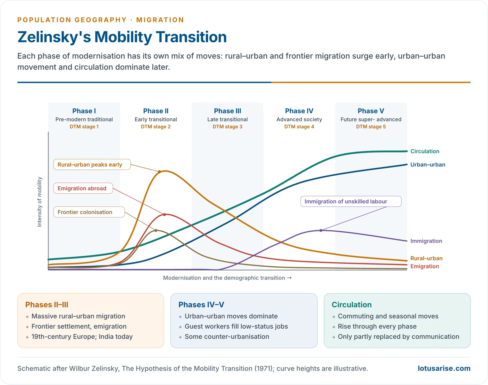
- Wilbur Zelinsky (1971) linked mobility to the demographic transition and to modernisation.
- His hypothesis: there are patterned regularities in the growth of personal mobility through space and time, and these are an essential part of modernisation.
- He tracked five forms of mobility together:
- international migration;
- frontier (colonisation) migration;
- rural–urban migration;
- urban–urban and intra-urban migration;
- circulation (commuting, seasonal and other non-permanent moves).
| Phase | Society | Mobility pattern |
|---|---|---|
| I | Pre-modern traditional | Little residential migration; limited circulation (pilgrimage, trade, war) |
| II | Early transitional | Massive rural–urban migration; frontier colonisation; emigration abroad; circulation rises |
| III | Late transitional | Rural–urban migration slackens; emigration falls; circulation grows and diversifies |
| IV | Advanced | Urban–urban and intra-urban moves dominate; immigration of unskilled labour; heavy circulation |
| V | Future super-advanced | Almost all moves inter- or intra-urban; some circulation replaced by communication; strict control of immigration |
- Pattern across phases:
- Dominant flows shift from rural–rural to rural–urban, then urban–urban, and finally include urban–rural (counter-urbanisation).
- International and regional migration rise in the early transitional phase, when population grows fast and transport improves. They decline later as immigration controls tighten and regional disparities narrow. Where rural development lags, regional migration persists longer.
- Rural–urban migration peaks in the early and middle phases, when industry and cities expand. It slackens once rural conditions improve and cities saturate.
- Urban–urban movement, from small towns to cities to metros, grows continuously through the later phases (Tier-2 cities to Delhi, Mumbai, Bengaluru).
- Congestion, high living costs and pollution start an urban–rural counter-current in advanced societies, as in the USA and Britain from the 1970s.
- Historical fit:
- Phase II matches 19th-century Europe: rural exodus to industrial towns and mass emigration to the Americas and Australia.
- Phase IV matches post-war Western Europe: urban–urban moves plus guest workers from Turkey, North Africa and southern Europe.
- India today combines phase II–III traits (large rural–urban and circular migration) with phase IV traits in its metros.
- Urban–urban flows grew fastest between 2001 and 2011, and counter-urbanisation remains weak.
- Evaluation:
- Strengths:
- The first model to tie migration systematically to the demographic and development transition.
- It treats all forms of mobility together, including circulation, and invites comparison between countries.
- Limitations:
- It assumes a single, linear path based on the Western experience.
- It neglects forced migration, politics and global inequality.
- Its prediction that communication would replace circulation has only partly held: remote work exists, but circulation and international migration have kept rising.
- Strengths:
Economic and Structural Theories
Dual-Sector and Neoclassical Models
- W. Arthur Lewis (1954), the dual-sector model:
- A traditional sector has surplus labour with near-zero marginal product.
- A modern urban-industrial sector absorbs it at a constant wage until the surplus is exhausted (the Lewis turning point).
- Rural–urban migration is the mechanism of structural transformation. Gustav Ranis and John Fei (1961) refined the model.
- Neoclassical macro theory:
- Migration results from geographical differences in wages, caused by unequal supply of and demand for labour.
- Labour flows from low-wage to high-wage regions until wages converge. Migration is an equilibrating force.
- Neoclassical micro theory (human capital):
- Larry A. Sjaastad (1962) treated migration as an investment in human capital.
- A person moves if the present value of expected returns exceeds the costs: money, psychic costs and earnings forgone.
- This explains why the young and educated move most: they have the longest pay-off period.
- Critique: wages have not converged between India’s states or between South Asia and the Gulf, and the poorest, who gain most, often move least because they cannot meet the costs.
- Indian application: India’s slow absorption of farm labour into manufacturing means the Lewis transfer has run mostly into construction and informal services, not factories. Agriculture still employed about 46% of workers in PLFS 2023–24, so the surplus-labour reservoir remains large.
Todaro and Harris–Todaro Models
- Michael P. Todaro (1969) and John R. Harris and Michael P. Todaro (1970) asked why rural people keep moving to cities despite high urban unemployment:
- Migrants respond to expected, not actual, urban income.
- Expected income = urban wage × probability of getting a formal job.
- Migration continues until expected urban income equals rural income. Equilibrium is reached with urban unemployment and a swollen informal sector.
- A simple illustration: if the urban formal wage is twice the rural wage but only a third of job-seekers find formal work, the expected urban income is below the rural wage and migration should slow; if the chance rises to two-thirds, migration resumes even while many remain jobless.
- Todaro framed the decision over a lifetime: a migrant may accept years in the informal sector for the prospect of a formal job later.
- Implications:
- Creating urban jobs can raise unemployment, because each new job attracts several migrants (the Todaro paradox).
- Rural development and narrowing rural–urban gaps are better policy than urban job creation alone. This logic underlies MGNREGA, PURA and the Shyama Prasad Mukherji Rurban Mission in India.
- Critique:
- It assumes a single decision-maker and ignores remittances, networks and family strategy.
- Gary Fields (1975) showed that the urban informal sector is not just a waiting room; it is a place of work and of job search in its own right.
New Economics of Labour Migration (NELM)
- Oded Stark and David E. Bloom (1985) shifted the unit of decision from the individual to the household.
- Families send one or more members away to diversify income and insure against risk: crop failure, price shocks, illness, and missing credit and insurance markets.
- Remittances are central. They finance consumption, debt repayment, housing, schooling and farm investment.
- Relative deprivation (Stark and J. Edward Taylor, 1989): households migrate to improve their position relative to their neighbours, not only in absolute terms. Migration can therefore occur without a wage gap.
- Indian examples:
- One son from a Bihar household works in Punjab or Surat while the rest farm.
- Kerala households diversify through Gulf migration; remittances built the state’s “Gulf houses” and financed its consumer economy.
- Critique: it assumes harmony within the household and pays little attention to gender inequalities in who decides and who goes.
Dual (Segmented) Labour Market Theory
- Michael J. Piore (1979) located the cause in the destination economy:
- Advanced economies have a primary sector (secure, well-paid jobs) and a secondary sector (unstable, low-status, low-paid jobs).
- Native workers avoid the secondary sector, so employers recruit migrants. International migration is demand-driven and built into modern industrial economies.
- It explains active recruitment: Turkish Gastarbeiter in Germany, South Asian construction workers in the Gulf, and care and domestic workers from the Philippines.
- Critique: it ignores sending-country factors and treats migrants as passive.
World Systems and Historical-Structural Views
- Building on Immanuel Wallerstein (1974), writers such as Saskia Sassen (1988) argued that migration follows the penetration of capitalism into peripheral societies.
- Land consolidation, mechanised farming and factory jobs uproot people, while the same material, cultural and transport links carry them towards the core.
- Migration therefore flows along colonial and economic ties:
- South Asians to Britain;
- North Africans to France;
- Filipinos to the USA;
- global cities concentrate the demand.
- Marxian and dependency writers see migration as a transfer of labour that serves capital at the core and keeps the periphery underdeveloped, a view that also fits the colonial indentured labour system.
- Critique: it is too deterministic and leaves little room for individual agency or for South–South flows.
Network, Systems and Perpetuation
Network Theory and Chain Migration
- Migrant networks are ties of kinship, friendship and shared origin linking migrants, former migrants and non-migrants.
- They lower the costs and risks of moving: information, a place to stay, a first job, a loan.
- This leads to chain migration and to clustering by origin:
- Malayalis in the Gulf;
- Gujaratis in East Africa and the UK;
- Punjabis in Canada;
- Odia workers in Surat’s textile and diamond units.
- Networks are a form of social capital. Once a network reaches a threshold, migration becomes less selective, because the costs fall for everyone in the community.
Migration Systems Theory
- Akin L. Mabogunje (1970) treated rural–urban migration in Africa as a system: origin and destination linked by flows of people, money, goods and information, with feedback loops and control sub-systems (rural family, urban employers, the state).
- Return information from successful migrants encourages more moves. Failure discourages them.
- Countries tied by history, trade and policy form migration systems, such as the Gulf–South Asia and North America–Mexico systems.
Cumulative Causation
- Gunnar Myrdal (1957) proposed cumulative causation. Douglas S. Massey (1990) applied it to migration.
- Each act of migration alters the social context in ways that make further migration more likely:
- Remittance-led inequality creates relative deprivation in non-migrant households.
- Land is bought by migrants and left fallow or used less intensively.
- A culture of migration forms, where moving becomes a rite of passage.
- Human capital is redistributed.
- Jobs at the destination are labelled as migrant jobs.
- Migration thus becomes self-perpetuating, even after its original cause weakens.
Institutional Theory
- Once flows begin, recruitment agencies, smugglers, lawyers, NGOs and diaspora bodies grow up to serve them.
- They sustain migration independently of the original wage gap. Kerala’s and Punjab’s recruitment and visa-consultancy industries are examples.
- Douglas S. Massey and colleagues (1993) combined these strands in an influential review of international migration theory.
Transnationalism
- Nina Glick Schiller, Linda Basch and Cristina Szanton Blanc (1992) described migrants who live across borders, keeping economic, social and political ties with home while settling abroad, as in today’s diasporas.
- Cheap travel, the internet, mobile money and dual-status schemes such as India’s Overseas Citizen of India card have multiplied such ties.
Models of Forced Migration
- Economic theories assume choice. Forced migration needs its own frameworks.
- Egon F. Kunz (1973), the kinetic model of refugee flight:
- Anticipatory refugees leave early, before the crisis peaks, usually with resources, skills and some choice of destination.
- Acute refugees flee in mass, under immediate threat, with little choice of where they go.
- The Partition of 1947 and the flight from East Pakistan in 1971 were acute movements. Professionals who leave a country quietly as political tension builds are anticipatory refugees.
- Anthony H. Richmond (1993) placed all moves on a continuum from proactive (largely voluntary) to reactive (largely forced). Most real flows mix choice and compulsion.
- Development-induced displacement (dams, mines, industrial corridors, such as the Sardar Sarovar and Hirakud projects) and disaster displacement are now studied as forms of forced migration.
Contemporary Perspectives
- Aspirations–capabilities framework (Hein de Haas, 2021):
- Migration depends on both the aspiration and the capability to move.
- Development at first raises emigration, because more people can afford to leave (the migration hump). It falls only at higher income levels.
- Environmental and climate migration:
- Slow-onset change (drought, salinity, sea-level rise) and sudden disasters act through existing economic and social channels.
- Examples: the Sundarbans, the Sahel, small island states.
- Feminisation of migration: more women now move independently for work, especially in nursing, domestic and care work.
- Skilled, student and digital mobility: IT professionals, the H-1B route, platform and gig work.
- The state as gatekeeper: visas, points systems, labour mobility agreements and deportations shape flows as much as wages do.
Comparative Evaluation
| Theory | Unit | Driver | Explains well | Weakness |
|---|---|---|---|---|
| Neoclassical | Individual | Wage gap | Direction of flows | Ignores households, structures |
| Todaro | Individual | Expected income | Urban unemployment with migration | Single decision-maker |
| NELM | Household | Risk, relative deprivation | Remittances, moves without wage gaps | Neglects structure |
| Dual labour market | Destination economy | Demand for cheap labour | Recruitment, guest-worker flows | Ignores origin |
| World systems | Global economy | Capitalist penetration | Colonial and core–periphery links | Too deterministic |
| Network / cumulative causation | Community | Social capital, feedback | Persistence of flows | Weak on how flows begin |
- The theories are complementary:
- Macro theories explain where flows originate.
- Micro theories explain who moves.
- Meso theories explain why flows persist after the original causes fade.
- Most early theories were built on voluntary, economic, male migration. Forced migration, marriage migration and family moves needed separate frameworks.
- The migration–development debate has swung like a pendulum:
- 1950s–1960s, optimism: migration transfers labour, capital and ideas and speeds development (Lewis, neoclassical theory).
- 1970s–1980s, pessimism: brain drain, dependence on remittances and the decline of sending regions (world systems, cumulative causation).
- 1990s onward, a pluralist view: outcomes depend on context. Remittances, return migrants, diaspora investment and the “brain gain” effect (the prospect of emigration encourages more people to acquire skills) can help development, but only where origin-country policies and institutions allow.
- India illustrates both sides: Kerala’s remittance-led social development, and the shortage of doctors and nurses in parts of India as health workers leave.
- Applied to India:
- Lewis and Todaro fit rural–urban migration into the informal sector.
- NELM fits remittance households in Bihar, eastern Uttar Pradesh and Kerala.
- Network theory fits chain migration to Surat, Tiruppur and the Gulf.
- Dual labour market theory fits Indian workers in the GCC.
- Distance decay still governs the largely intra-district pattern of Indian migration.





There is a gravity model but I think there is another gravity model is needed that is John q Stewart model
Very quality level content. I really appreciate it.
Plz add stuart gravity model also. Thanks.
Very helpful notes ❤️