Ecosystem: Structure, Functions, Energy Flow and Biogeochemical Cycles

• An ecosystem is a functional unit of nature in which a community of living organisms interacts with its non-living environment, so that energy flows through it in one direction and matter circulates within it in cycles.
  • The term was put into print by Arthur George Tansley (1935), who borrowed it from his young colleague Arthur Roy Clapham. Tansley wanted a word that treated organisms and their physical surroundings as one interacting physical system, not as a plant community with a backdrop.
• Every ecosystem has a structure (what it is made of and how its parts are arranged) and functions (what it does: fix energy, pass it along food chains, cycle nutrients and regulate itself).
• Ecosystems exist at every scale, from a drop of pond water or a rotting log to a forest, a lake or an ocean basin. The biosphere is the largest of them, the single global ecosystem.
• For a geographer the concept is valuable because it is monistic: climate, soil, landforms, plants, animals and people sit in one framework, and human use of land can be read as a change in the flows and stores of the system. That is why the ecosystem became a core unit of environmental geography.

The Ecosystem Concept

Meaning and definitions

• Arthur George Tansley (1935) defined ecosystems as a category of physical systems made of organisms and inorganic components in a relatively stable equilibrium, open, and of various sizes and kinds.
  • He split the whole into the biome (the complex of plants and animals of a place) and the habitat (its physical environment), and insisted that the two are interacting factors that, in a mature system, are in approximate balance.
• Raymond Laurel Lindeman (1942) gave the concept its energy basis. In his study of Cedar Bog Lake in Minnesota, he described the ecosystem as any system of physical, chemical and biological processes within a space–time unit of any size, and grouped organisms into trophic levels linked by energy transfer.
• F. Raymond Fosberg (1963) called it a functioning, interacting system of one or more organisms and their effective environment, physical and biological.
• Eugene P. Odum (1971) gave the definition most quoted today:
  • any unit that includes all the organisms (the community) of an area interacting with the physical environment, so that a flow of energy leads to a clearly defined trophic structure, biotic diversity and material cycles within the system.
• Physical geographers stress the systems view: the ecosystem is the sum of all organisms and substances of an area, a basic example of an open system with inputs and outputs of energy and matter, used to build and maintain living structure (biomass).
• A working definition: an ecosystem is a space–time unit of the Earth’s surface in which the total assemblage of organisms and the abiotic environment, powered mainly by solar energy, interact through energy flow and nutrient cycling.

The ecosystem as an open system

System	Energy crosses the boundary	Matter crosses the boundary	Example
Isolated	No	No	Approximated only in the laboratory
Closed	Yes	No (after the initial input)	The Earth as a whole, almost exactly
Open	Yes	Yes	Every real ecosystem: a pond, a forest, a city

• The Earth is effectively closed for matter but open for energy. Sunlight comes in and heat radiates out, while the planet’s atoms are recycled again and again. That is why energy must flow and matter must cycle.
• Ecosystems are open systems. A forest receives sunlight, rain, dust and migrating animals, and loses heat, water, dissolved nutrients and sediment.
  • When inputs and outputs balance, the system is in a steady state (dynamic equilibrium): its stores stay roughly constant even though material passes through all the time.
  • When the balance is upset, for example by deforestation or nutrient overload, the stores change and the system shifts. This is the basis of ecological imbalance.
• For convenience, an ecosystem can be studied as a black box: only the input and output variables are measured, and the internal workings are ignored to reduce complexity.

Properties of an ecosystem

• Space–time unit: it occupies a definite area and is studied over a definite time.
• Three components: energy, biotic (biome) and abiotic (habitat). The energy component is often grouped with the abiotic one.
• Interactions run between the biotic and abiotic parts and among the organisms themselves.
• Open system, powered chiefly by solar energy, with a few systems at deep-sea vents and caves running on chemical energy.
• Linked by cycles: energy flow, the water cycle, nutrient (biogeochemical) cycles and the sediment cycle bind the parts together.
• Productivity: every ecosystem builds organic matter at a characteristic rate per unit area per unit time.
• Self-regulation: it tends towards a relatively stable equilibrium unless a limiting factor is disturbed.
• Development: it changes through time by ecological succession towards a mature, more stable state.
• Scale: from a tree hole to the whole biosphere, so ecosystems can be ranked in orders by size.
• Natural resource system: forests, fisheries, grasslands and croplands are ecosystems that people harvest.

Types of ecosystems

Basis	Types	Examples
Habitat	Terrestrial; aquatic (freshwater and marine)	Forest, grassland, desert, tundra, mountain; river, lake, wetland; open ocean, estuary, coral reef
Origin	Natural; human-made (artificial)	Rainforest, mangrove; cropland, plantation, aquarium, city
Use (E. P. Odum, 1959)	Cultivated; non-cultivated	Rice, wheat, sugarcane fields; forest, tall-grass and short-grass ecosystems
Scale	Micro, meso, macro (biome), global	Tree hole, pond; forest; tropical rainforest biome; biosphere
Energy source	Solar-powered; chemosynthetic	Almost all ecosystems; hydrothermal vents and cold seeps

• Terrestrial ecosystems follow climate. At the largest scale they form the biomes of the world: tropical rainforest, savanna, desert, temperate grassland, temperate forest, taiga and tundra, plus mountain systems.
• Freshwater ecosystems are lotic (running water: rivers, streams) or lentic (standing water: lakes, ponds), with wetlands between land and water.
• Marine ecosystems cover about 71% of the Earth’s surface and are zoned in two ways:
  • By light: the sunlit photic zone (to about 200 m), where all photosynthesis happens, and the dark aphotic zone below, which lives on sinking organic matter (“marine snow“).
  • By position: the pelagic (open water) and benthic (sea floor) realms; the neritic zone over the continental shelf and the oceanic zone beyond it.
  • Productivity is patchy: coral reefs, estuaries, upwelling zones and shelves are highly productive, while the nutrient-poor open ocean is close to a biological desert per square metre.
  • Indian examples include the coral reefs of the Gulf of Mannar, Lakshadweep and the Andaman and Nicobar Islands, the Sundarbans mangrove–estuary system, and the summer upwelling off the Kerala coast that feeds the oil-sardine fishery.
• Chemosynthetic ecosystems were discovered at the Galápagos Rift in 1977. Bacteria oxidise hydrogen sulphide from hydrothermal vents and support tube worms, clams and crabs in total darkness.

The biosphere as an ecosystem

• The biosphere is the life-supporting layer of the Earth: the biologically inhabited parts of the lithosphere, hydrosphere and atmosphere, where life exists without any protective device.
  • Vertical extent: life is found from the floor of the deepest ocean trenches (about 11 km down) to microbes lofted several kilometres into the atmosphere. Most organisms, however, live in a thin film within a few hundred metres above and below the land and sea surface.
  • Upper limit is set by falling oxygen, moisture, temperature and air pressure. The lower limit on land is the depth of the deepest roots, burrows and weathered rock; in the oceans, by light for producers and by food supply for the rest.
• It qualifies as an ecosystem because it has all the parts and processes of one:
  • an abiotic component: land and soil, air and water;
  • a biotic component: plants, animals (including people) and micro-organisms;
  • an energy component: solar radiation, with a minor geothermal and chemical input;
  • interactions among them through large-scale cycles of energy, water, carbon, nutrients and sediment.
• It is an open system for energy and a closed one for matter. As long as energy input balances heat output and the cycles keep running, the biospheric system stays in dynamic equilibrium. When a critical limit is crossed, environmental and ecological problems follow.
• Sub-systems:
  • Terrestrial: a plant system, an animal system and a soil system, linked by cyclic pathways of energy and matter.
  • Aquatic: a plant system (mainly phytoplankton), an animal system and a nutrient system in the water.
  • The soil system is the biosphere’s biological furnace and factory. It is the zone where dead matter is broken down, nutrients are stored, and roots take them up again; it also houses the largest share of the planet’s species.
• Plants dominate living matter. Of about 550 billion tonnes of carbon held in all life on Earth, plants hold roughly 80% and bacteria most of the rest. Animals hold only about 2 billion tonnes, and humans a tiny 0.06 billion tonnes (2018 census of the biosphere).
• Modifiers of the biospheric ecosystem:
  • Physical: temperature change, water flow, fire, mining, construction;
  • Chemical: changes in the make-up of air, water and soil, for example CO2 build-up or acid deposition;
  • Biological: cropping patterns, changes in species density and distribution, and genetic manipulation.
• The biosphere regulates itself to some degree. James Lovelock’s Gaia hypothesis (developed with Lynn Margulis in the 1970s) proposed that life helps keep the atmosphere, oceans and climate within the bounds life needs. It is debated as a strict theory but has shaped Earth system science.

Structure of an Ecosystem

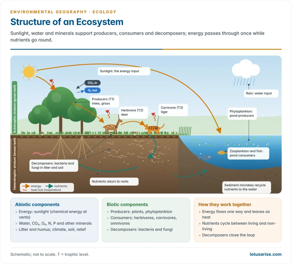
• Structure means the composition of the biological community (species, numbers, biomass), the quantity and distribution of non-living materials, and the range of conditions (temperature, light, moisture) in which the community lives.

Abiotic components

• Energy: solar radiation is the basic input. Only visible light (photosynthetically active radiation) drives photosynthesis; the rest heats the system. Chemical energy in reduced compounds drives the vent and seep communities.
• Inorganic substances: water, carbon dioxide, oxygen, nitrogen, and mineral nutrients such as phosphorus, potassium, calcium, sulphur and trace elements, held in air, water, rock and soil.
  • The amount of these materials present in the system at a given time is called the standing state.
• Organic compounds: dead organic matter (litter, humus, dissolved organic matter) that links the living and non-living parts.
• Physical factors: the ecological factors of climate (temperature, light, rainfall, humidity, wind), soil (texture, pH, moisture) and topography (altitude, slope, aspect), each acting on organisms within limits of tolerance.

Biotic components

• Producers (autotrophs) make their own food from inorganic materials.
  • Photoautotrophs (green plants, algae, cyanobacteria, phytoplankton) use light: 6CO2 + 6H2O + light → C6H12O6 + 6O2.
  • Chemoautotrophs (sulphur, iron and nitrifying bacteria) obtain energy by oxidising inorganic compounds such as hydrogen sulphide, ammonia or ferrous iron, and use it to fix CO2. They do not use ready-made organic matter.
  • Producers are the link between the abiotic and the biotic worlds: they pull carbon from the air and nutrients from the soil into living tissue.
• Consumers (heterotrophs) depend directly or indirectly on producers.
  • Herbivores (primary consumers): deer, cattle, grasshoppers, zooplankton.
  • Carnivores: secondary consumers that eat herbivores (frog, fox) and tertiary consumers that eat other carnivores (snake, hawk, tiger).
  • Omnivores feed at several levels; humans are the most important example.
  • Parasites live on or in a living host; detritivores (earthworms, termites, millipedes, crabs) eat dead organic matter.
  • By mode of feeding, consumers are holozoic (ingesting food through a mouth), parasitic or saprotrophic (absorbing dissolved organic matter from dead material).
• Decomposers (saprotrophs), mainly bacteria and fungi, break dead tissue down to simple inorganic forms by secreting enzymes and absorbing the products.
  • They close the nutrient loop. Without them, nutrients would stay locked in dead bodies and production would stop.

Functional group	Nutrition	Role	Examples
Abiotic elements	Not applicable	Habitat, energy and raw materials	Sunlight, water, CO2, minerals, humus
Producers	Autotrophic	Fix energy; turn inorganic into organic matter	Grass, trees, phytoplankton, vent bacteria
Consumers	Heterotrophic (holozoic, parasitic)	Transfer and use energy; regulate producers	Deer, tiger, zooplankton, tapeworm
Decomposers	Heterotrophic (saprotrophic)	Break down dead matter; release nutrients	Bacteria, fungi

Spatial arrangement: autotrophic and heterotrophic strata

• Eugene P. Odum described two layers in most ecosystems:
  • an upper autotrophic stratum (the “green belt“): the canopy or the sunlit surface water, where light is fixed;
  • a lower heterotrophic stratum (the “brown belt“): the soil, litter and sediments, where organic matter is used, rearranged and decomposed.
• Vertical stratification of a forest (emergents, canopy, understorey, shrub, herb and litter layers) and of a lake (littoral, limnetic and profundal zones) multiplies the niches available.
• Standing crop is the biomass present at a given moment, usually expressed as dry weight per unit area.

Functions of an Ecosystem

• An ecosystem performs six linked functions:
  1. Primary production: fixing solar energy as organic matter;
  2. Energy flow: passing that energy along food chains;
  3. Decomposition: breaking down dead matter;
  4. Nutrient cycling: circulating elements between living and non-living stores;
  5. Regulation: feedback control that keeps the system near a steady state;
  6. Development: change through succession.
• Energy flow is one-way and non-cyclic, while materials cycle. Energy flow is also the motor of nutrient cycling: every movement of matter through living organisms is driven by the energy they obtain.

Productivity

Primary productivity

• Productivity is the rate at which organic matter (or energy) is built up per unit area per unit time: grams of dry matter, grams of carbon or kilocalories per square metre per year.
  • Production is the amount produced over a stated period. Biomass is the amount present at one time, the standing crop. A grassland can have low biomass but high productivity; an old forest has huge biomass but modest net growth.
• Gross primary productivity (GPP): the total rate of photosynthesis, including the organic matter that the plants burn in their own respiration.
• Net primary productivity (NPP): what is left after the plants’ own respiration (Ra) is met: NPP = GPP − Ra.
  • NPP is the energy actually available to herbivores and decomposers, so it sets the ceiling for all life above trophic level 1.
  • In most ecosystems plants respire roughly half of GPP.
• Net ecosystem productivity (NEP): NPP minus the respiration of all heterotrophs (Rh): NEP = NPP − Rh. A positive NEP means the ecosystem is a carbon sink; a negative value means it is a source.
• Photosynthetic efficiency is low. Plants convert only about 1–2% of the sunlight falling on them into GPP during the growing season, and well under 1% averaged over the globe and the year.

Secondary productivity

• Secondary productivity is the rate at which consumers form new tissue from the food they assimilate.
  • Consumers do not fix energy; they only convert and reassemble it. Their production is therefore always far smaller than the NPP on which it rests.

Factors controlling productivity

• Light and temperature set the length and intensity of the growing season.
• Water is the main control on land: production rises with rainfall up to roughly 2,500 mm a year.
• Nutrients control the sea: nitrogen, phosphorus and iron are scarce in the open ocean, so upwelling zones and shelf seas fed by rivers and mixing are the productive waters.
• Biological factors: grazing pressure, competition, mutualism (for example root nodules and mycorrhizae) and the age of the stand.
• Whichever factor is in shortest supply limits production: water in hot deserts, light and temperature in the polar lands, nutrients in the open ocean.

Global patterns of productivity

Ecosystem	Mean NPP (g dry matter/m²/yr)	Note
Coral reefs	2,500	Highest per unit area
Tropical rainforest	2,200	Largest total land production
Swamps and marshes	2,000	Very high; small area
Estuaries	1,500	Nutrient trap of rivers and tides
Temperate deciduous forest	1,200	Seasonal
Savanna	900	Fire and grazing
Boreal forest	800	Short season
Cultivated land	650	Varies with inputs
Temperate grassland	600	Water-limited
Upwelling zones	500	Richest open-sea waters
Continental shelf	360	Moderate
Tundra and alpine	140	Cold-limited
Open ocean	125	Nutrient-poor
Desert scrub	90	Water-limited
Extreme desert, rock, ice	3	Almost none

• Figures are the classic world compilation of Robert H. Whittaker and Gene E. Likens (1975), which put the world mean at about 333 g/m²/yr, about 773 on land and 152 in the oceans.
• Modern satellite estimates put global NPP at about 105 billion tonnes of carbon a year, split almost equally: about 56 on land and 49 in the oceans (Christopher Field and colleagues, 1998).
  • The ocean paradox: per square metre the ocean is about a fifth as productive as the land, yet it matches the land in total because it covers 71% of the globe. Its producers are microscopic, fast-growing phytoplankton with tiny standing biomass.
• E. P. Odum (1959) grouped the world into three productivity belts:
  • High: shallow waters, moist tropical and temperate forests, alluvial plains and intensively farmed land;
  • Intermediate: grasslands, shallow lakes and ordinary farmland;
  • Low: deserts, the deep open ocean and polar ice wastes.
• The latitudinal trend: productivity falls from the humid tropics towards the poles with falling radiation and temperature, and drops sharply into dry belts.
• India: productivity is highest in the Western Ghats and north-eastern rainforests, the Sundarbans mangroves and irrigated Indo-Gangetic croplands, and lowest in the Thar and the cold desert of Ladakh.
• Human appropriation: people now use or remove about a quarter of the planet’s potential NPP through harvest, grazing, fire and land-use change. This is a measure of human dominance over the biosphere.

Food chains, trophic levels and food webs

Trophic levels

• A trophic level (from the Greek trophe, nourishment) is the position an organism occupies in the feeding sequence, counted in steps from the producers.
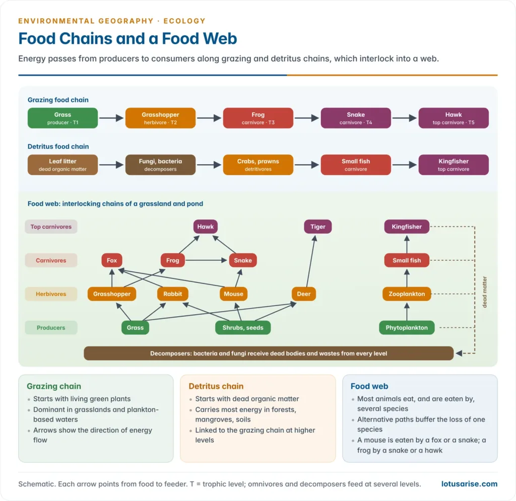
  • T1: producers; T2: herbivores (primary consumers); T3: primary carnivores (secondary consumers); T4: secondary carnivores (tertiary consumers); T5: top carnivores.
  • Raymond Lindeman (1942) showed that organisms can be grouped into such more or less discrete levels, each depending on the one below for energy.
• An organism can occupy more than one level. A bear eating berries is at T2 and eating salmon is at T4; humans feed at T2 to T4. Decomposers draw energy from every level.

Food chains

• A food chain is the sequence of organisms through which food energy passes, each eating the one before it. The idea was popularised by Charles Sutherland Elton (1927).
• Food chains are short, usually four or five links, because energy shrinks at every step.

Type	Starts with	Sequence (example)	Where it dominates
Grazing (predator) chain	Living green plants	Grass → grasshopper → frog → snake → hawk	Grasslands, plankton-based waters
Detritus chain	Dead organic matter	Mangrove leaf litter → fungi and bacteria → crabs, prawns → fish → kingfisher	Forests, mangroves, the deep sea, soils
Parasitic chain	A host	Tree → bark beetles → parasitic wasps	Runs from larger to smaller organisms

• Further examples:
  • Pond: phytoplankton → zooplankton → small fish → large fish → kingfisher or otter;
  • Ocean: diatoms → copepods → herring → seal → killer whale;
  • Indian grassland: grass → chital → tiger; grass → blackbuck → Indian wolf.
• Grazing and detritus chains are joined. Dung, carcasses and uneaten plants of the grazing chain feed the detritus chain, and detritivores such as earthworms are eaten by birds of the grazing chain.
• In most terrestrial ecosystems the detritus chain carries more energy. In forests, well over 90% of NPP is never eaten alive; it falls as litter and is consumed by decomposers. In aquatic systems herbivores eat about half of annual primary production, roughly three times the share eaten on land (Helene Cyr and Michael Pace, 1993).

Food webs

• A food web is the network of interlocking food chains in an ecosystem, formed because most species eat several kinds of food and are eaten by several predators.
• Classic illustrations:
  • Arctic: grasses feed caribou, hares and lemmings; these are eaten by wolves, foxes and people; in the sea, diatoms feed crustaceans, which feed fish, seals, walruses and whales, on which polar bears and people depend.
  • North Sea herring: an adult herring can reach diatoms through several routes, via arrow worms, sea butterflies or several species of copepod.
• Why webs matter:
  • They offer alternative pathways for energy. The loss of one prey species can be absorbed by switching to another.
  • Complex webs tend to buffer populations against fluctuations. The relationship is not simple, as the stability section below shows.
  • Webs explain ripple effects: a change at one node travels to many others.

Ecological pyramids

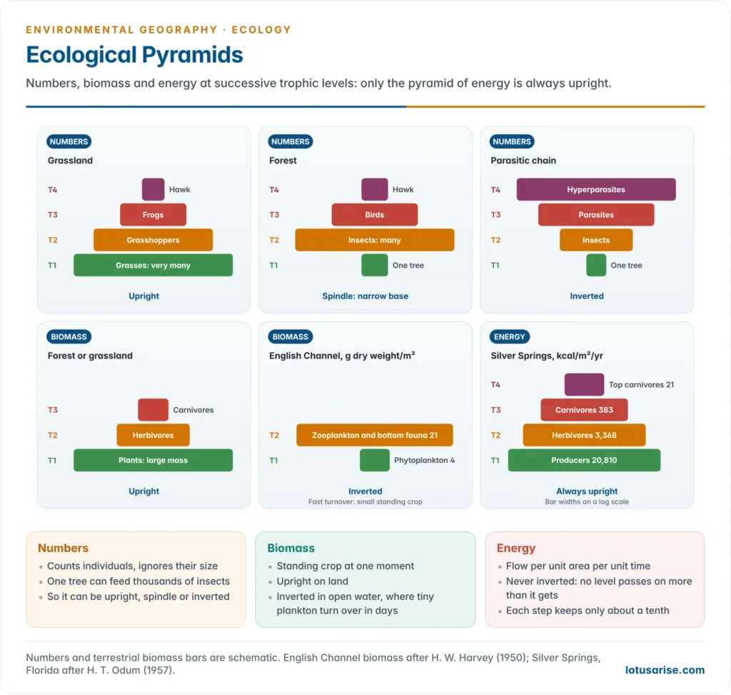
• An ecological pyramid shows the trophic structure of an ecosystem as stacked bars, one for each trophic level, with the producers at the base. Charles Elton (1927) first drew the pyramid of numbers, so these are also called Eltonian pyramids.
• Three kinds are drawn, each with its own logic.

Pyramid	Measures	Usual shape	Exceptions
Numbers	Individuals at each level per unit area	Upright: many grasses, fewer grasshoppers, a few frogs, one hawk	Spindle in a forest (one tree, many insects); fully inverted in a parasitic chain (one tree, many insects, more parasites)
Biomass	Standing crop (dry weight per unit area) at one time	Upright on land: a large plant mass supports a smaller animal mass	Inverted in open water: in the English Channel, about 4 g/m² of phytoplankton supported about 21 g/m² of zooplankton and bottom animals
Energy	Energy flowing through each level per unit area per unit time (kcal/m²/yr)	Always upright	None: no level can pass on more energy than it receives

• Why the biomass pyramid inverts in the sea: phytoplankton grow and divide in days and are eaten almost as fast, so a small standing crop with a rapid turnover feeds a larger, slow-growing mass of animals. A snapshot of biomass misses that rate.
• The energy pyramid is the most informative, because it measures flow over time. Howard Thomas Odum’s (1957) study of Silver Springs, Florida gave the classic figures, in kcal/m²/yr:
  • producers about 20,810 (gross production), herbivores 3,368, carnivores 383 and top carnivores 21, with decomposers processing about 5,060.
• Limitations of pyramids:
  • They ignore organisms that feed at several levels and the detritus pathway, which often carries most of the energy.
  • Numbers pyramids ignore size; biomass pyramids ignore turnover rate.
  • They describe a single ecosystem at one time, and seasonal changes can alter the shape.

Energy flow

Energy and the laws of thermodynamics

• The first law of thermodynamics: energy is neither created nor destroyed, only changed in form.
  • In an ecosystem, light energy becomes chemical energy in photosynthesis, and chemical energy becomes mechanical work and heat in respiration. The total input always equals the total output plus the change in storage.
• The second law of thermodynamics: every transformation degrades some energy to heat, which is dispersed and cannot do further work. Entropy rises.
  • At every transfer between trophic levels, most of the energy is lost as heat through respiration, so less is available at each higher level.
• Consequence: energy flow is unidirectional and non-cyclic. It enters as light and leaves as heat; it is never recycled. Ecosystems survive only because the Sun keeps supplying new energy.
• Biosynthesis (building tissue) stores energy; biodegradation (respiration and decay) releases it as heat.

The path of energy through an ecosystem

• Of the sunlight reaching vegetation, most is reflected or turned straight into heat and evaporation; plants fix only a small fraction as GPP.
• At each trophic level, the energy taken in is divided:
  • part is not assimilated and leaves as faeces, urine or uneaten material, which feeds decomposers;
  • part is respired to fuel the organism’s work (moving, hunting, keeping warm, reproducing) and is lost as heat;
  • the remainder becomes new tissue (growth and reproduction), and only this is available to the next level.
• Three pathways therefore leave each level:
  1. Upward, to the next trophic level (and, for omnivores like humans, directly from lower levels as well);
  2. Sideways, to decomposers as dead bodies and wastes;
  3. Outward, as heat from respiration, lost to the atmosphere and space.

Lindeman’s trophic-dynamic concept and the ten per cent law

• Lindeman (1942) treated each trophic level as an energy store and measured the transfers between them. This trophic-dynamic approach turned community ecology into a science of energy budgets.
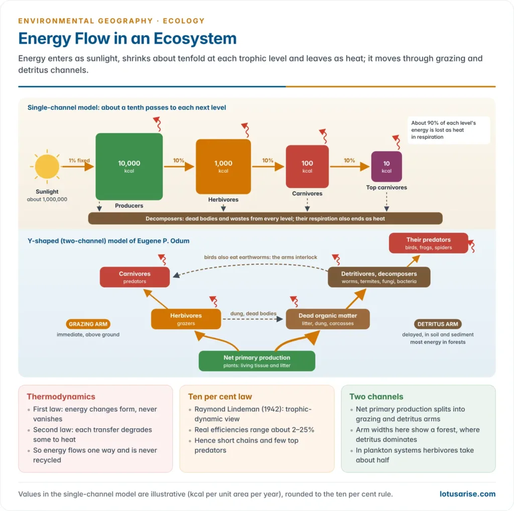
• The ten per cent law: on average, only about 10% of the energy at one trophic level is converted into tissue at the next; about 90% is lost.
  • So 10,000 kcal of plant energy supports about 1,000 kcal of herbivores, 100 kcal of carnivores and 10 kcal of top carnivores.
  • The figure is a rule of thumb, not a constant. Measured transfer efficiencies range from about 2% to 25%, and average close to 10% in aquatic food webs.

Efficiency	Meaning	Typical pattern
Ecological (Lindeman) efficiency	Production at level n ÷ production at level n − 1	About 10%, range 2–25%
Assimilation efficiency	Energy absorbed ÷ energy eaten	Carnivores about 80% (meat is digestible); herbivores 20–60% (cellulose and lignin are not)
Production efficiency	New tissue ÷ energy assimilated	Ectotherms (insects, fish) 10–40%; endotherms (birds, mammals) 1–3%, because keeping warm costs energy

• Consequences of the ten per cent law:
  • Food chains are short, seldom beyond four or five links: too little energy remains to support another level.
  • Top predators are few and range widely. A tiger needs a large territory of prey-rich forest, which is why their numbers fall first when habitat shrinks.
  • Eating lower in the chain feeds more people. A plant-based diet feeds several times more people from the same land than one based on grain-fed meat.
  • Persistent toxins concentrate upward while energy thins out. This biomagnification of DDT and mercury harms top predators most.

Models of energy flow

• Single-channel (linear) model: energy passes in a straight line from producers to herbivores to carnivores, with losses as heat at each step. It shows the thermodynamic logic but ignores detritus.
• Y-shaped (two-channel) model of Eugene P. Odum: NPP divides into two arms:
  • a grazing arm (living plants → herbivores → carnivores);
  • a detritus arm (dead organic matter → decomposers and detritivores → their predators).
  • The arms are linked at the base (both start from NPP) and at higher levels (detritivores are eaten by carnivores of the grazing arm).
  • It is more realistic because it separates time and space: grazing is immediate and above ground, while detritus use is delayed and mostly in the soil and sediments. It also shows how the balance between the arms differs between forests (detritus-dominated) and plankton systems (grazing-heavy).
• Universal model (E. P. Odum, 1968): a single compartment model for any living unit (plant, animal, population or trophic level). Ingested energy is split into assimilated and unassimilated parts, and assimilated energy into respiration and production.

Decomposition

• Decomposition breaks complex dead organic matter into CO2, water and mineral nutrients. It is carried out mainly by bacteria and fungi, helped by detritivores.
• Stages:
  • Fragmentation: detritivores such as earthworms, termites and millipedes chew litter into small pieces, increasing the surface area.
  • Leaching: water-soluble nutrients wash down into the soil.
  • Catabolism: bacterial and fungal enzymes break the material into simpler compounds.
  • Humification: a dark, amorphous, slowly decaying colloid called humus forms, a long-term nutrient store.
  • Mineralisation: humus is slowly broken down further, releasing inorganic nutrients such as ammonium and phosphate.
• Controls:
  • Climate: it is fastest in warm, moist, well-aerated conditions and slowest in cold or waterlogged ones.
  • Litter chemistry: litter rich in nitrogen and sugars decays fast, while litter rich in lignin and chitin decays slowly.
• Geographic contrast:
  • In the tropical rainforest, litter vanishes within months. Most nutrients are held in the living biomass, and soils are poor, so clearing the forest strips the nutrient capital.
  • In the taiga and tundra, decay is so slow that organic matter piles up as raw humus and peat, and permafrost soils store vast amounts of carbon.

Biogeochemical Cycles

Concept

• Biogeochemical cycles are the cyclic pathways by which chemical elements move from the non-living environment (air, water, rock, soil) into living organisms and back again.
  • Each cycle has a biotic phase (bio), a geological phase (geo) and chemical changes between forms (chemical).
  • They can be pictured as a set of compartments (stores, reservoirs) linked by flows (fluxes).
• Two kinds of pool are distinguished in each cycle:
  • a large, slow-moving reservoir pool, mostly non-biological: the atmosphere for nitrogen, rocks for phosphorus;
  • a smaller, fast-moving exchange (cycling) pool, shuttling between organisms and their immediate surroundings.
• Residence time is the average time an atom spends in a store: store ÷ flux. Water stays about 9 days in the atmosphere but thousands of years in the deep ocean; carbon stays millions of years in limestone.
• Nutrients needed by life:
  • Macronutrients, needed in large amounts: carbon, hydrogen and oxygen (about 90% of dry organic matter), plus nitrogen, phosphorus, potassium, calcium, magnesium and sulphur;
  • Micronutrients (trace elements), needed in tiny amounts: iron, manganese, zinc, copper, boron, molybdenum, chlorine, nickel, and cobalt for some organisms.
• The generalised cycle: elements from the atmospheric phase (brought down by rain and fixation) and the sedimentary phase (released by weathering) gather in the soil pool. Plants take them up in solution through their roots and build them into tissue. They then pass along the food chain and return to the soil when wastes, litter and dead bodies are decomposed, or when vegetation burns.
  • Losses are by leaching to groundwater, by erosion and runoff to the sea, and by gaseous escape. These are made good by new inputs.

Basis	Gaseous cycles	Sedimentary cycles
Main reservoir	Atmosphere (and ocean)	Earth’s crust: rocks, sediments, soil
Examples	Carbon, nitrogen, oxygen, water (hydrogen)	Phosphorus, sulphur (mixed), calcium, potassium, iron
Speed	Fast; global mixing through the air	Slow; tied to weathering, erosion and uplift
Self-regulation	Good: large atmospheric buffer evens out local shortages	Poor: losses to deep-sea sediments are effectively permanent on human timescales
Typical human impact	Carbon and nitrogen loading of the air; climate change	Mining and fertiliser runoff; eutrophication

The water cycle

• Water is the medium of all other cycles. It dissolves nutrients, carries them to roots and to the sea, and is split in photosynthesis.
• Hydrogen enters and leaves the biosphere mainly as water, so the hydrogen cycle is studied as the hydrological cycle: evaporation, transport by winds, condensation, precipitation, interception, infiltration, runoff and return to the sea.
• Stores: about 97% of the Earth’s water is in the oceans, about 2% in ice caps and glaciers, and well under 1% in groundwater, lakes, soils, rivers, the atmosphere and living things.
• Annual fluxes (thousand km³ a year, recent estimates):
  • Over the oceans, evaporation of about 413 exceeds precipitation of about 373.
  • Over the land, precipitation of about 113 exceeds evapotranspiration of about 73.
  • The surplus of about 40 is carried from sea to land as vapour and returns as river runoff and groundwater flow.
• Vegetation links the water and nutrient cycles. Evapotranspiration returns about two-thirds of the land’s rain to the air, most of it through plant transpiration, and forest clearing reduces local rainfall recycling, as in the Amazon.

The carbon cycle

• Carbon is the backbone of all organic molecules and makes up about half the dry weight of living matter. Its movements are closely tied to the flow of energy: photosynthesis stores energy in carbon bonds, and respiration releases both.
• Carbon exists in three phases:
  • Gaseous: CO2 and methane (CH4) in the air;
  • Dissolved: CO2, bicarbonate (HCO3−) and carbonate (CO3²−) in water;
  • Solid: organic matter, fossil fuels (coal, oil, gas, peat), and carbonate rocks and shells (CaCO3).

The fast (biological) carbon cycle

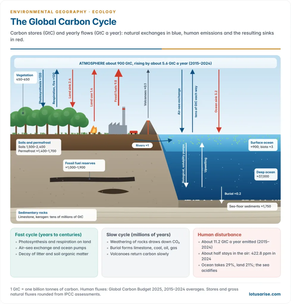
• Photosynthesis on land draws down about 120 billion tonnes of carbon (GtC) a year, and respiration by plants, animals and decomposers, together with fire, returns almost the same amount.
• Air–sea exchange: CO2 dissolves in cold, high-latitude waters and degasses from warm, upwelling tropical waters. Gross exchange is a few tens of GtC each way every year.
• The ocean moves carbon downward by three “pumps”:
  • Solubility pump: cold, dense water absorbs CO2 and sinks into the deep ocean;
  • Biological pump: phytoplankton fix CO2, and their remains sink as marine snow, carrying carbon to depth;
  • Carbonate pump: plankton and corals build calcium carbonate shells, part of which settles as sediment.
  • A microbial carbon pump also turns organic carbon into forms that bacteria cannot readily break down, which persist in deep water for thousands of years.
• Uptake is both donor-controlled and recipient-controlled. The rate depends on the CO2 concentration in the air (the donor) and on the density and activity of plants (the recipient), along with light, water and nutrients.

The slow (geological) carbon cycle

• Over millions of years, carbon moves between rocks and the surface:
  • Chemical weathering of silicate and carbonate rocks consumes CO2. Rivers carry bicarbonate to the sea, where it is locked into limestone.
  • Burial of organic matter in swamps and sea-floor muds forms coal, oil, gas and kerogen.
  • Volcanoes and metamorphism return carbon to the air, but slowly, at well under 1 GtC a year, about one hundredth of human emissions.
• Sedimentary rocks hold by far the largest store, tens of millions of GtC, with a residence time of hundreds of millions of years.

Store	Approximate size (GtC)
Atmosphere (2025, about 425 ppm CO2)	about 900
Land vegetation	450–650
Soils (excluding permafrost)	1,500–2,400
Permafrost	about 1,400–1,700
Surface ocean	about 900
Intermediate and deep ocean	about 37,000
Fossil fuel reserves	about 1,000–1,900
Sedimentary rocks	tens of millions

Human disturbance of the carbon cycle

• Atmospheric CO2 has risen from about 278 ppm before industrialisation to 422.8 ppm in 2024 and a projected 425.6 ppm in 2025.
• Global Carbon Budget 2025, average annual flows for 2015–2024:
  • Sources: fossil fuels and cement about 9.8 GtC, plus land-use change (mostly tropical deforestation) about 1.4 GtC: a total of about 11.2 GtC a year.
  • Where it went: about 5.6 GtC stayed in the atmosphere (about half), 3.2 GtC went into the ocean (about 29%) and 2.4 GtC into the land (about 21%).
  • 2024 set a record: fossil emissions of 10.3 GtC, and an atmospheric rise of 3.7 ppm, the largest on record, because hot El Niño conditions, droughts and fires weakened the land sink.
  • The remaining carbon budget for 1.5 °C was about 170 billion tonnes of CO2, roughly four years of current emissions.
• Consequences:
  • an enhanced greenhouse effect and global warming;
  • ocean acidification: surface pH has fallen from about 8.2 to 8.1 since pre-industrial times, roughly a 30% rise in acidity, which threatens corals and shell-builders;
  • a risk of feedbacks as warming thaws permafrost and dries forests, which could turn sinks into sources.
• India: the forest and tree cover held an estimated 7,285 million tonnes of carbon in 2023. Mangroves, seagrasses and salt marshes (blue carbon ecosystems) store carbon at very high rates per hectare. Enlarging these sinks is part of India’s path to net zero by 2070.

The oxygen cycle

• Oxygen is chemically very active and occurs as free O2 (about 21% of the air), as water, as CO2, and in oxides and carbonates of the crust, which hold by far the largest amount.
• It is closely coupled to the carbon cycle:
  • Release: photosynthesis splits water and releases O2. Marine phytoplankton produce about half of it, and land plants the rest.
  • Consumption: respiration of all organisms, decomposition, combustion of wood and fossil fuels, and oxidation of minerals (rusting of iron, weathering).
• Origin: the early atmosphere had almost no free oxygen. It accumulated after cyanobacteria began photosynthesising, rising sharply in the Great Oxidation Event about 2.4 billion years ago. Its presence also built the ozone layer that made life on land possible.
• Is oxygen running out? No. The atmosphere’s vast O2 store changes only slowly. Measurements do show a small, steady decline in atmospheric O2 as fossil fuels burn. The more serious loss is deoxygenation of the oceans and the spread of coastal dead zones.

The nitrogen cycle

• Nitrogen is an essential part of amino acids, proteins, nucleic acids (DNA, RNA) and chlorophyll.
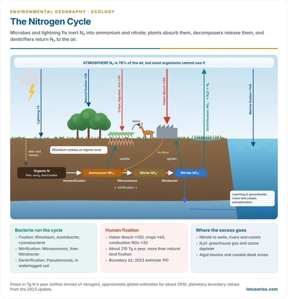
• The atmosphere is 78% N2, the largest store. Yet N2 is almost inert, because of its strong triple bond, and most organisms cannot use it. Nitrogen must first be “fixed” into ammonium (NH4+) or nitrate (NO3−), so it is often the limiting nutrient on land.
• The cycle is driven by bacteria. Every conversion between inorganic forms is carried out mainly by prokaryotes (bacteria, archaea and cyanobacteria).

Steps of the nitrogen cycle

1. Nitrogen fixation: N2 → ammonia (NH3) or nitrate.
   • Atmospheric fixation: lightning joins N2 and O2 into nitrogen oxides. These form nitric acid in rain, and reach the soil as nitrate.
   • Biological fixation by the enzyme nitrogenase:
     • symbiotic: Rhizobium in root nodules of legumes (pulses, soybean, groundnut, clover, alfalfa) and Frankia in alder and casuarina;
     • free-living: Azotobacter (aerobic), Clostridium (anaerobic) and cyanobacteria such as Anabaena and Nostoc. Anabaena lives with the water fern Azolla in rice fields.
     • In the oceans, cyanobacteria such as Trichodesmium fix nitrogen.
   • Industrial fixation: the Haber–Bosch process (Fritz Haber, 1909; scaled up by Carl Bosch, 1913) combines N2 with hydrogen at high temperature and pressure to make ammonia for fertilisers.
2. Assimilation: plants absorb ammonium and nitrate through their roots and build them into proteins. Animals obtain nitrogen by eating plants or other animals.
3. Ammonification (mineralisation): decomposers turn the organic nitrogen of dead bodies, urea and uric acid into ammonia/ammonium.
4. Nitrification: two groups of chemoautotrophic bacteria oxidise ammonium in two steps:
   • NH4+ → nitrite (NO2−) by Nitrosomonas (and ammonia-oxidising archaea);
   • NO2− → nitrate (NO3−) by Nitrobacter.
   • Nitrate is the form most plants take up, but it is highly mobile and easily leached.
5. Denitrification: in waterlogged, oxygen-poor soils and sediments, bacteria such as Pseudomonas use nitrate in place of oxygen and reduce it, step by step, to nitrous oxide (N2O) and N2, which returns to the air. Anammox bacteria also convert ammonium and nitrite directly to N2 in oxygen-free waters.
6. Losses occur by leaching of nitrate to groundwater, runoff to rivers and the sea, and volatilisation of ammonia from manure and urea.

Human alteration of the nitrogen cycle

• People now fix more nitrogen than all natural land processes together. Natural biological fixation on land is about 58 million tonnes (Tg) of N a year, and lightning about 5 Tg. Human activities add about 210 Tg: about 120 Tg from Haber–Bosch, about 60 Tg from cultivated legumes and rice, and about 30 Tg from combustion.
• The planetary boundary for intentionally fixed nitrogen is about 62 Tg N a year. The 2023 assessment put the current figure at about 190 Tg, about three times the safe limit.
• Consequences:
  • eutrophication of lakes, rivers and coasts, and coastal dead zones;
  • nitrate in drinking water;
  • N2O, a greenhouse gas about 270 times as potent as CO2 over a century, and now the leading ozone-depleting emission;
  • acid deposition from nitrogen oxides;
  • loss of plant diversity where nitrogen-loving species take over.
• In India, heavy and urea-skewed fertiliser use and low nitrogen-use efficiency in rice–wheat systems add to nitrate pollution of groundwater in Punjab and Haryana. Neem-coated urea (2015), soil health cards and pulses and Azolla in rotations aim to raise efficiency.

The phosphorus cycle

• Phosphorus is part of DNA, RNA and ATP (the energy currency of cells), of cell membranes, and of bones and teeth. It is often the limiting nutrient in freshwater.
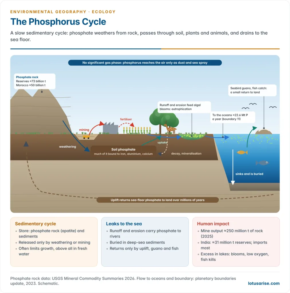
• It is a sedimentary cycle with no significant gaseous phase. Phosphorus enters the air only as dust and sea spray.
• The pathway:
  • Weathering of phosphate rocks (apatite) releases phosphate into the soil.
  • Plants take up dissolved inorganic phosphate and build it into organic compounds, which pass along the food chain.
  • Decomposition and mineralisation of wastes and dead bodies return phosphate to the soil.
  • Phosphate binds tightly to iron, aluminium and calcium in soils, so only a small fraction is available to plants at any time.
• The cycle leaks towards the sea. Runoff and erosion carry phosphate to rivers and oceans, where it sinks into deep-sea sediments.
  • It returns to the land only when those sediments are uplifted by tectonic movement, over millions of years.
  • Small, local returns come through seabird guano (as on the Pacific coast of South America), fish eaten on land, and sea spray.
  • On a human timescale the cycle is effectively one-way, from land to sea.
• Human impact:
  • Mining of phosphate rock for fertiliser has multiplied the flow. World mine output was about 250 million tonnes in 2025. Reserves of about 73 billion tonnes are highly concentrated, with Morocco holding about 50 billion tonnes. India has only about 31 million tonnes and imports most of its phosphatic fertiliser and raw material.
  • Phosphorus flowing from fresh water to the oceans, about 22.6 million tonnes a year, is about twice the planetary boundary of 11 million tonnes.
  • Eutrophication: excess phosphate from fertilisers, detergents and sewage causes algal blooms, oxygen depletion and fish kills in lakes and reservoirs, such as Bengaluru’s Bellandur lake.

The sulphur cycle

• Sulphur is a component of the amino acids cysteine and methionine and of many vitamins. Its cycle is mixed: a large sedimentary store in rocks (gypsum, pyrite) and a lively gaseous phase.
• Natural pathways:
  • weathering of rocks releases sulphate (SO4²−), which plants absorb;
  • decomposition releases hydrogen sulphide (H2S) in waterlogged soils and marshes;
  • sulphur bacteria oxidise H2S to sulphate, while others reduce sulphate back to H2S in oxygen-free muds;
  • volcanoes emit SO2;
  • marine phytoplankton release dimethyl sulphide (DMS), which forms sulphate aerosols that seed clouds.
• Human impact: burning coal and oil and smelting ores release SO2, which forms sulphuric acid and causes acid rain. Sulphate aerosols also cool the climate and damage health. Emission controls such as flue-gas desulphurisation in coal plants reduce the load.

Regulation, Stability and Ecosystem Services

Homeostasis and cybernetics

• Homeostasis is the ability of an ecosystem to resist change and return to a steady state after a disturbance, through built-in self-regulation.
  • Cybernetics, the science of control and communication systems founded by Norbert Wiener (1948), gives the language: ecosystems are controlled not by a central “thermostat” but by diffuse feedback among populations and processes.
• Negative feedback dampens change and keeps the system near its set point.
  • Example: if favourable weather lets an insect population boom beyond its food supply, food runs short, competition and predation rise, many die, and the population falls back.
  • The predator–prey cycles of lynx and snowshoe hare follow the same logic.
• Positive feedback amplifies change and can push a system across a threshold.
  • Example: warming melts sea ice, the darker sea absorbs more heat, and more ice melts.
• The homeostatic plateau: within a certain range of stress, negative feedback keeps the system stable. Beyond it, positive feedback takes over and the system may collapse or shift to a different state.

Stability and resilience

• Ecosystem stability means a balance between production and consumption of each element and a broadly constant structure, even though individual organisms and atoms are constantly replaced.

Kind of stability	Meaning	Example
Constancy	Little change in numbers or biomass over time	Climax tropical rainforest
Resistance	Ability to withstand a disturbance without changing	A mature forest resists a dry year
Resilience	Speed and ability to recover after disturbance	Grassland regrows quickly after fire
Cyclical (elastic) stability	Regular oscillation around a mean in response to periodic change	Seasonal plankton cycles; predator–prey cycles

• Crawford Stanley Holling (1973) distinguished engineering resilience (how fast a system returns to its old state) from ecological resilience (how much disturbance it can absorb before it flips to a different state).
  • Examples of flips: a clear lake becoming turbid and algae-dominated; a coral reef becoming a seaweed-covered rubble; a rainforest drying into a degraded savanna. Such regime shifts are hard to reverse.
• The diversity–stability debate:
  • Robert MacArthur (1955) argued that more links in a food web give more alternative paths for energy, and so more stability.
  • Charles Elton (1958) noted that simple systems (islands, monocultures) are more easily invaded and suffer pest outbreaks.
  • Eugene P. Odum linked high diversity and homeostasis to mature (climax) communities.
  • Robert May (1973) showed mathematically that randomly assembled complex webs can be less stable. Real webs are not random, but this prompted more careful thinking.
  • David Tilman’s long-term grassland experiments at Cedar Creek, Minnesota (1990s) found that more diverse plots kept their productivity steadier through drought.
  • Current view: diversity tends to stabilise ecosystem functions (total production, nutrient retention) even when individual populations fluctuate. This is the insurance effect of having several species able to do the same job.
• Two models of equilibrium:
  • The equilibrium model sees ecosystems returning quickly to a balanced state after disturbance.
  • The non-equilibrium model sees frequent disturbance (fire, floods, storms) keeping many systems in perpetual change. Patchy, shifting mosaics are the norm.
• Ecosystem instability arises when change is too fast or too large for the system’s resilience.
  • Natural causes: climatic change, volcanic eruptions, invasive pathogens.
  • Human causes: removing or replacing native vegetation and animals; introducing exotic species; changing land use; adding pesticides and herbicides; altering the composition of the air; and manipulating water and nutrient flows.
  • Example: in parts of the Himalaya, clear-felling followed by heavy grazing exposed slopes to erosion and nutrient loss, so that forests could not regenerate. This is a classic case of instability that the Chipko movement resisted.

“The web of life is seamless”: ripple effects

• Because every species is tied to others through food webs, nutrient cycles and habitat, a change at one point ripples through the whole. Ecosystems are not machines with spare parts that can be removed without consequence.
• Trophic cascades: removing or adding a top predator changes herbivore numbers, which changes the vegetation, which changes soils, streams and other species.
  • Sea otters, urchins and kelp: where otters were hunted out along the North Pacific coast, sea urchins multiplied and grazed away the kelp forests. Where otters returned, the kelp recovered (James Estes and John Palmisano, 1974).
  • Wolves in Yellowstone: after reintroduction in 1995–96, elk numbers and behaviour changed, and willows and aspens regenerated along some streams. The strength of the cascade is still debated, a reminder that ecosystems respond in complex ways.
  • Tigers and leopards in Indian forests help keep deer and wild-pig numbers in check, which lets forest seedlings regenerate.
• Keystone species have an effect far larger than their abundance. The term comes from Robert T. Paine, who removed the starfish Pisaster from rocky shores in Washington in the 1960s and saw diversity collapse as mussels took over.
  • Other examples: figs in tropical forests (fruit in lean seasons); elephants (opening forests, dispersing seeds); beavers (creating wetlands); and ecosystem engineers such as termites and corals.
• Indian vultures, a ripple through people:
  • The veterinary painkiller diclofenac in cattle carcasses caused kidney failure in vultures. Gyps vulture populations fell by more than 95% from the 1990s.
  • Uncleared carcasses fed feral dogs and rats, raising rabies risk and polluting water. A 2024 economic study linked the collapse to about half a million additional human deaths between 2000 and 2005.
  • Veterinary diclofenac was banned in 2006, and conservation breeding continues.
• Other ripples:
  • Pollinator decline threatens crop yields.
  • Invasive species such as Lantana camara and water hyacinth displace native plants and choke waterways.
  • DDT moved up food chains and thinned the eggshells of birds of prey.
  • Ripples also run through cycles, not just webs: fertiliser on Punjab fields becomes nitrate in wells, and soil eroded from Himalayan slopes silts reservoirs downstream.
  • Multiplied across regions, such ripples add up to global and regional ecological imbalances.

Ecosystem services

• Ecosystem services are the benefits people obtain from ecosystems.
  • The Millennium Ecosystem Assessment (MEA), called for by the UN Secretary-General Kofi Annan in 2000 and published in 2005, drew on more than 1,300 experts. It classified these benefits into four categories and linked them to human well-being.

Category	What it means	Examples
Provisioning	Products obtained from ecosystems	Food, fresh water, timber, fuelwood, fibre, medicinal plants, genetic resources
Regulating	Benefits from the regulation of ecosystem processes	Climate and carbon storage, flood and storm protection (mangroves), water purification, pollination, pest and disease control, erosion control
Cultural	Non-material benefits	Sacred groves and rivers, tourism and recreation, aesthetic and spiritual value, traditional knowledge
Supporting	Processes needed for all other services	Primary production, soil formation, nutrient cycling, the water cycle, habitat

• Constituents of well-being in the MEA are security, basic materials for a good life, health, good social relations and freedom of choice and action.
• Key MEA findings:
  • Humans changed ecosystems more rapidly and extensively in the second half of the 20th century than in any comparable period.
  • About 60% of the services examined (15 of 24) were being degraded or used unsustainably.
  • The costs fall most heavily on the poor, who depend directly on forests, fisheries and commons.
• Valuing services:
  • Robert Costanza and colleagues (1997) estimated the world’s ecosystem services at about US$33 trillion a year, more than the global GNP of the time. A 2014 update raised this to about US$125 trillion a year.
  • The Economics of Ecosystems and Biodiversity (TEEB) carried valuation into policy and ecosystem management.
• IPBES (2019) reframed services as nature’s contributions to people, giving weight to cultural and indigenous views of nature. It found three-quarters of the land surface and two-thirds of the ocean significantly altered by people.
• Indian examples:
  • Mangroves of the Sundarbans and Odisha’s Bhitarkanika reduced storm damage in the 1999 Odisha super cyclone and later cyclones.
  • Chilika lake recovered its fishery and Irrawaddy dolphins after a new mouth to the sea was opened in 2000. It was removed from the Ramsar Montreux Record in 2002.
  • Himalayan forests, glaciers and wetlands regulate water for the plains: the highland–lowland link that makes mountain ecosystems so valuable.