- Island biogeography studies why islands hold the number and kinds of species they do. Its central model, the equilibrium theory of island biogeography, explains species number as a balance between the arrival of new species and the loss of resident ones.
- The theory, built by Robert MacArthur and Edward O. Wilson (1963, 1967), applies to any habitat island: a mountaintop, a lake, a forest fragment or a national park surrounded by farmland.
- It sits alongside the great continental pattern of richness, the latitudinal diversity gradient, in which species numbers rise from the poles to the tropics.
The Theory of Island Biogeography

Islands as natural laboratories
- Islands are discrete, countable and replicated: each has a clear edge, a measurable area and a known distance from the nearest source of colonists. That makes them ideal for testing ideas about distribution.
- Charles Darwin (Galápagos) and Alfred Russel Wallace (Malay Archipelago) built their ideas of evolution partly on island evidence.
| Type | Origin | Biota | Examples |
|---|---|---|---|
| Oceanic islands | Volcanic or coral; never joined to a continent | Few groups, colonised only by sea or air; high endemism; no native land mammals except bats on the most remote | Hawaii, Galápagos, Lakshadweep, Barren Island |
| Continental (land-bridge) islands | Parts of a continental shelf, cut off by rising sea level | Sample of the mainland biota; species lost since isolation | Sri Lanka, Britain, Borneo, Taiwan |
| Habitat islands | Patches of habitat in a “sea” of different land | Species of the patch, isolated by unsuitable surroundings | Mountaintops, lakes, caves, forest fragments, protected areas |
- Typical features of island biotas:
- Disharmony: whole groups are missing (large mammals, amphibians, freshwater fish) because they cannot cross the sea.
- High endemism: isolation lets populations diverge into new species, the core of endemism.
- Adaptive radiation: one colonist fills many empty niches, as with Darwin’s finches of the Galápagos and the Hawaiian honeycreepers.
- The island rule: large mammals tend to dwarf (the extinct dwarf elephants of Mediterranean islands) and small ones to grow large (giant rats, the Komodo dragon).
- Loss of dispersal and defence: flightless birds such as the dodo and the kiwi.
- Extreme vulnerability: invasive species drive about 90% of extinctions on islands (IPBES, 2023).
The species–area relation
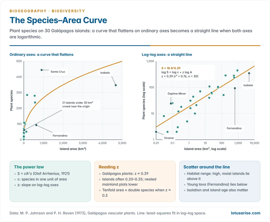
- Larger areas hold more species. Olof Arrhenius (1921) expressed this as a power law:
- S = cA^z, where S is the number of species, A the area, c a constant (species in one unit of area) and z the slope.
- Taking logarithms gives a straight line: log S = log c + z log A. On ordinary axes the curve rises steeply and then flattens.
- Typical slopes: z is commonly about 0.20–0.35 for true islands and lower, about 0.1–0.2, for nested samples within a continent.
- Philip Darlington’s (1957) rule of thumb: a tenfold increase in area doubles the number of species (z ≈ 0.3).
- Frank Preston (1962) derived a z near 0.26 from the way individuals are shared among species.
- A 2006 meta-analysis of nearly 700 curves found that slopes depend more on the group studied and the scale than on island versus mainland.
- Galápagos plants: across 30 islands, from 0.01 km² to Isabela’s 4,669 km², plant species rise from 2 to 444; the best-fit line is about S = 18A^0.39 (data of Johnson and Raven, 1973).
- Why larger areas hold more species:
- More habitats (Isabela and Fernandina have high volcanoes with moist uplands; small islets are bare lava and shore).
- Larger populations, which are less likely to die out.
- Bigger targets for colonists and room for speciation.
- Sampling: a larger area simply samples more individuals and therefore more species.
- Use in conservation: with z = 0.25, losing 90% of a habitat cuts its species to 0.1^0.25, about 56%, a loss of some 44%.
- Such projections can overestimate immediate extinctions, because a species dies out only when its last population goes; many survivors carry an extinction debt that is paid later.
MacArthur and Wilson’s equilibrium model
- Robert H. MacArthur and Edward O. Wilson proposed the model in An Equilibrium Theory of Insular Zoogeography (1963) and developed it in The Theory of Island Biogeography (1967).
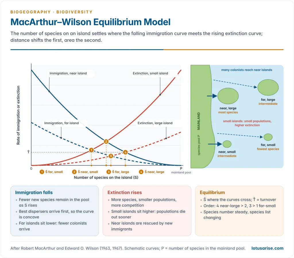
- Core claim: the number of species on an island settles at a dynamic equilibrium where the rate of immigration of new species equals the rate of extinction of resident species. The number stays roughly constant, but the list of species keeps changing (turnover).
- The immigration curve falls as the island fills:
- It starts at its maximum when the island is empty and reaches zero when all P species of the mainland pool are present.
- It is concave: the best dispersers arrive first, so the rate drops quickly at first and then slowly.
- The extinction curve rises as species accumulate:
- More species means more candidates for extinction, smaller average populations and more competition.
- It is concave upward for the same reasons.
- The equilibrium number (Ŝ) lies where the two curves cross; the height of the crossing is the turnover rate.
- Distance effect: islands far from the mainland receive fewer immigrants, so their immigration curve is lower and Ŝ smaller.
- Area effect: small islands hold small populations that die out more easily, so their extinction curve is higher and Ŝ smaller. Small islands are also smaller targets for colonists.
- If the curves are simplified to straight lines, with immigration falling from I₀ to zero and extinction rising from zero to E₀ at S = P, then Ŝ = P·I₀ / (I₀ + E₀).
| Island | Immigration | Extinction | Equilibrium richness |
|---|---|---|---|
| Near and large | High | Low | Highest |
| Near and small | High | High | Intermediate |
| Far and large | Low | Low | Intermediate |
| Far and small | Low | High | Lowest |
- r- and K-selection: the 1967 book also introduced these terms. The first colonists of an empty island tend to be r-strategists (good dispersers that breed fast), while later arrivals that win in crowded communities are K-strategists (strong competitors with fewer young).
- The model’s four predictions:
- richness rises with area and falls with isolation;
- richness on a disturbed or new island climbs back to the same equilibrium;
- at equilibrium there is continuous turnover of species;
- the time to reach equilibrium is predictable from the rates.
Testing the theory
Simberloff and Wilson’s mangrove experiment
- In 1966–67 Daniel Simberloff and Edward O. Wilson covered small red mangrove islets in the Florida Keys with tents and fumigated them with methyl bromide, removing all their insects, spiders and other arthropods.
- They then counted the recolonists for two years (results published in 1969 and 1970).
- Within about a year most islets were back to roughly their original number of species, as the theory predicts.
- The nearest islet recovered fastest and the most distant reached the lowest total, confirming the distance effect.
- The species lists differed from the originals and kept changing, confirming turnover.
- Island size could not be tested, because the islets were all much the same size.
Krakatau after 1883
- The eruption of Krakatau in August 1883 buried the remaining islands of the group under hot ash and sterilised them. In May 1884 the only living thing found was a spider.
- Plants arrived first by wind and sea: ferns and grasses by 1886, then strand and pioneer trees. Animal-dispersed plants increased from the 1920s, once fruit bats and fruit-eating birds had settled.
| Survey | Resident land bird species | Change |
|---|---|---|
| 1908 | 13 | First recorded colonists |
| 1919–21 | 28 | Rapid rise |
| 1932–34 | 29 | 34 species established in all, but 5 had died out |
| 1951–52 | 33 | Slow rise |
| 1984–85 | 35 | 14 new species and 8 losses since 1934 |
- Order of arrival: wind-borne spores and seeds first, sea-borne strand plants next, then birds, bats and the fruit trees they carry. Non-flying mammals other than rats remain few, a direct sign of dispersal filtering.
- Reading the record: MacArthur and Wilson took the near-flat bird count after about 1920 as an equilibrium with turnover. Later surveys showed that colonisation went on and that extinction was slower than predicted, partly because the forest itself was still maturing.
- A new volcano, Anak Krakatau, rose from the sea in 1927–30; its flank collapse on 22 December 2018 caused a deadly tsunami and reset its succession.
Other evidence
- Faunal relaxation on land-bridge islands: islands cut off by post-glacial sea-level rise have lost species since isolation, the smallest the most.
- National parks as islands: William Newmark (1987) found that the smallest parks of western North America had lost the largest share of their mammal species since their creation.
- Forest fragments: the Biological Dynamics of Forest Fragments Project near Manaus, begun in 1979 by Thomas Lovejoy, isolated 1, 10 and 100 ha fragments of rainforest. Army-ant-following birds vanished from the 1 and 10 ha fragments within two years.
- Isolation gradients: bird species decline steadily with distance from New Guinea across the islands of Melanesia and Polynesia, as the immigration curve predicts.
- Time to equilibrium: islands close to a source refill in years, as in the mangrove experiment; remote oceanic islands take thousands to millions of years and add species mainly by speciation in place.
Refinements and criticism
- Rescue effect (James Brown and Astrid Kodric-Brown, 1977): on islands close to the mainland, a stream of immigrants props up dwindling populations, lowering extinction. Immigration and extinction are therefore not independent.
- Target effect: larger islands intercept more colonists, so area raises immigration as well as lowering extinction.
- Small-island effect: on very small islets, richness varies with chance disturbance and habitat, not with area.
- Habitat diversity, not area itself, may be the real driver in many cases.
- Speciation is ignored. On large, remote islands new species arise in place (Hawaii, Galápagos). The general dynamic model of Robert J. Whittaker, Kostas Triantis and Richard Ladle (2008) adds speciation and the life cycle of a volcanic island, from emergence through peak size to erosion and submergence.
- All species are treated as equal, though a predator, a pollinator or a keystone tree matters far more than a beetle. Equilibrium is often never reached, because disturbance and climate change move the target.
- Turnover is hard to measure: casual visitors and missed species inflate or hide it.
- Metapopulation thinking grew from the model: Richard Levins (1969) described a species as a network of local populations that wink out and are refounded, the same immigration–extinction balance applied to patches of habitat.
- Value: despite its limits, the theory founded conservation biogeography, guided reserve design, and led to the study of fragmentation and metapopulations in human-modified landscapes.
Habitat Islands and Reserve Design
Habitat islands
- Any patch of habitat cut off by unsuitable land behaves like an island: mountaintops (sky islands), lakes and springs, caves, forest remnants in farmland, and protected areas surrounded by settlement.
- Habitat islands differ from true islands: the surrounding land is not empty sea. Some species cross farmland or plantations easily, and the matrix itself supplies weeds, predators and edge effects, so isolation is a matter of degree.
- Fragmentation turns continuous habitat into habitat islands. Fragments lose species over decades, the extinction debt, and suffer edge effects from wind, light, fire and weeds.
- Western Ghats sky islands: montane shola forest–grassland patches above about 1,400 m are separated by deep valleys and gaps such as the Palghat Gap.
- Their birds have diverged into two endemic genera described in 2017, Sholicola (shortwings) and Montecincla (laughingthrushes), with different species on different massifs.
- The Nilgiri tahr and many frogs and plants are confined to such peaks.
- Rainforest fragments on the Valparai plateau of the Anamalai Hills, isolated by tea and coffee estates, still shelter lion-tailed macaques and have been the focus of restoration since the early 2000s.
The SLOSS debate and reserve design principles
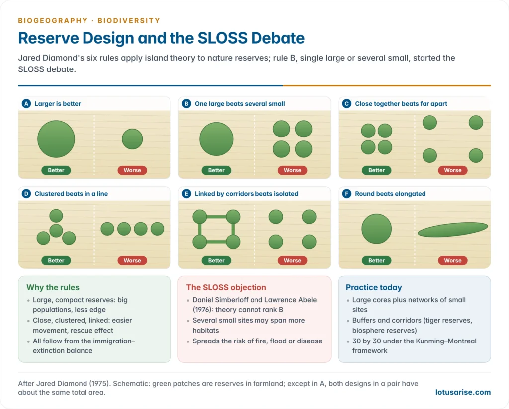
- Jared Diamond (1975), in The Island Dilemma, turned the theory into geometric rules for nature reserves:
- A larger reserve is better than a smaller one.
- A single large reserve is better than several small ones of the same total area.
- Reserves close together are better than reserves far apart.
- Reserves clustered together are better than reserves in a line.
- Reserves linked by corridors are better than isolated ones.
- A compact (round) reserve is better than an elongated one, as it has less edge.
- Daniel Simberloff and Lawrence Abele (1976) challenged rule 2: the theory does not say whether one large or several small reserves hold more species. That started the SLOSS (single large or several small) debate.
| Single large | Several small |
|---|---|
| Supports wide-ranging and large species (tiger, elephant) that need big home ranges | Can cover more habitat types and so more species in total |
| Larger populations, lower extinction risk | Spreads risk: one fire, flood or epidemic cannot destroy all |
| Less edge per unit area | Often cheaper and easier to acquire near people |
| Keeps natural processes (fire, flood, migration) intact | Fragments may be all that is left in farmland |
- Current view: both are needed. A 2020 review by Lenore Fahrig of empirical studies found that several small patches usually held as many or more species than few large ones of equal total area. Large cores remain essential for area-demanding species.
- Modern design combines large core areas, buffer zones, corridors and networks of smaller sites, as in UNESCO’s biosphere reserves (core, buffer and transition zones) and India’s tiger reserves and tiger corridors.
- The Kunming–Montreal Global Biodiversity Framework (2022) asks for 30% of land and sea to be conserved by 2030 in well-connected systems.
- Corridors are not free of cost: they can spread fire, disease and invasive species, and a narrow strip may be all edge. They work best when they carry real habitat and follow the routes animals already use.
- Shape and buffer: a round reserve with a buffer of compatible land use keeps edge effects away from its core; a long, thin reserve is mostly edge.
Patterns of Species Richness
The latitudinal diversity gradient
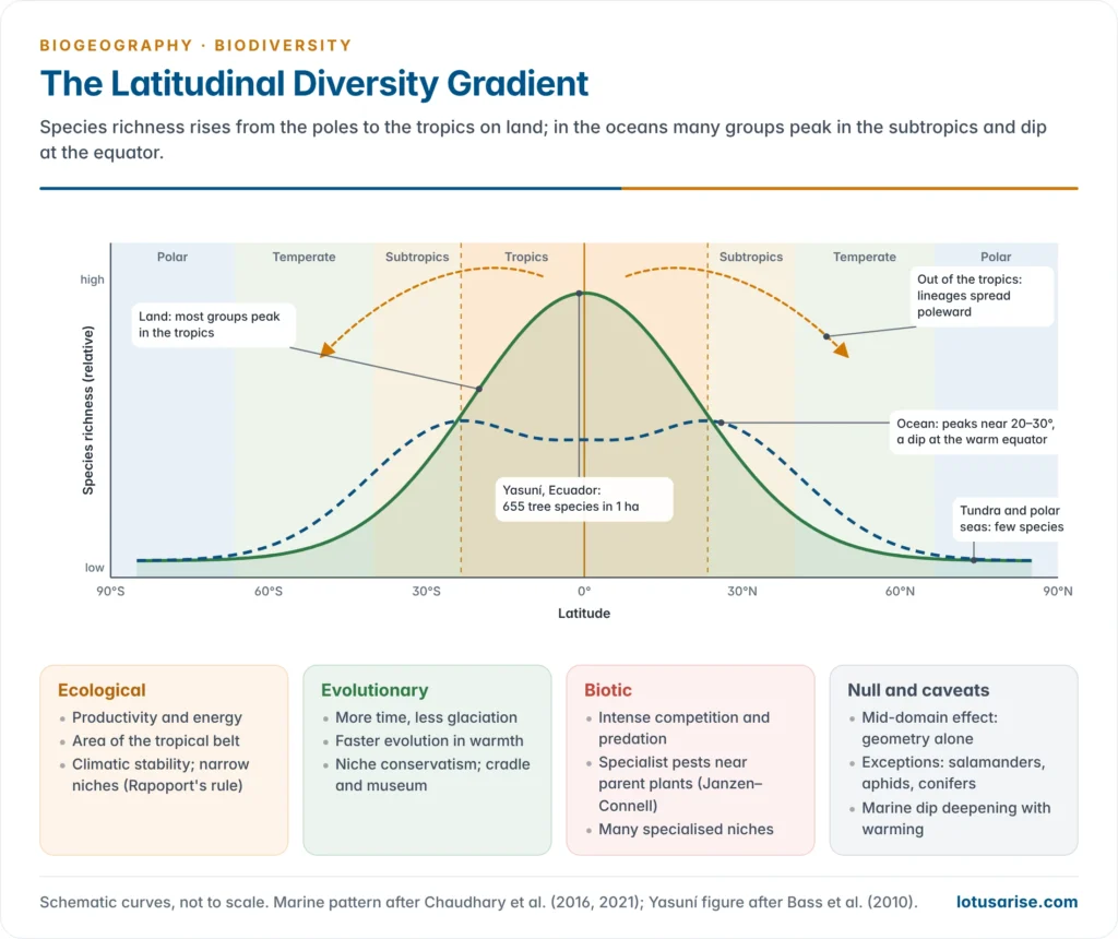
- Species richness is highest in the tropics and falls towards the poles. It is the oldest and most general pattern in biogeography, noted by Alexander von Humboldt and Alfred Russel Wallace (1878).
- It holds for most groups: trees, birds, mammals, amphibians, reptiles, ants, butterflies, freshwater fish and reef corals.
- An average upland hectare of Yasuní, Ecuador, holds about 655 tree species, more than are native to the United States and Canada together.
- Edward O. Wilson found 43 ant species on a single tree in the Peruvian Amazon, about as many as in the whole of the British Isles.
- Exceptions and variations:
- Some groups peak outside the tropics: salamanders (eastern North America), aphids, conifers and many seabirds.
- Marine species show a bimodal pattern, peaking at about 20–30° N and S with a dip at the warm equator. The dip has deepened with recent warming as species move poleward (Chaudhary and co-workers, 2021).
- In the fossil record the gradient was flatter in warm greenhouse periods and steepest in cold “icehouse” ones.
- On mountains, richness often peaks at middle elevations.
- India follows the gradient only loosely: the Western Ghats and the Eastern Himalaya, both tropical and wet, are hotspots, while the cold, dry trans-Himalaya and Thar are poorer. Rainfall and relief cut across latitude.
- Why the gradient matters:
- Most of the world’s species, and most of its biodiversity hotspots, lie in a tropical belt that is also losing forest fastest, so conservation effort is unevenly needed.
- Tropical species have narrow thermal tolerances, so even modest warming can push them past their limits, while temperate communities gain warm-adapted newcomers.
- The gradient also sets beta diversity: tropical communities change species rapidly over short distances, which is why the alpha, beta and gamma components differ so sharply between the tropics and high latitudes.
Hypotheses for the latitudinal gradient
| Hypothesis | Main idea | Proponents | Weakness |
|---|---|---|---|
| Time and stability | Tropics are older and were less disrupted by glaciation, so more species have accumulated | Alfred Russel Wallace (1878); Alfred Fischer (1960) | Tropics also changed in the Pleistocene (drier, cooler phases) |
| Area | Tropics form the largest climatically similar zone, so ranges are large, extinction low and speciation high | John Terborgh (1973); Michael Rosenzweig (1995) | Tundra and desert are also vast but poor |
| Productivity and energy | More sunlight, warmth and water support more individuals and so more species | G. Evelyn Hutchinson (1959); David Currie (1991) | Very productive places are not always richest |
| Seasonality and narrow niches | Stable climates allow narrow tolerances and finer division of resources; ranges shrink towards the equator (Rapoport’s rule) | George Stevens (1989) | Rapoport’s rule holds mainly in the northern hemisphere |
| Evolutionary speed | Warmth speeds metabolism, generation time and mutation, so speciation is faster | Klaus Rohde (1992); Andrew Allen, James Brown and James Gillooly (2002) | Rates differ widely among groups |
| Biotic interactions | Intense competition, predation and pest pressure keep any one species from dominating | Theodosius Dobzhansky (1950); Janzen–Connell effect | Hard to separate cause from effect |
| Tropical niche conservatism | Most groups arose in the tropics and few evolved cold tolerance | John Wiens and Michael Donoghue (2004) | Explains persistence, not origin |
| Out of the tropics | Tropics are both cradle (high origination) and museum (low extinction); lineages spread poleward without losing tropical presence | David Jablonski, Kaustuv Roy and James Valentine (2006) | Based mainly on marine fossils |
| Mid-domain effect | Ranges placed at random within a bounded domain overlap most in the middle | Robert Colwell and George Hurtt (1994) | A null model; ignores climate |
- Synthesis: no single cause explains the gradient. Ecological factors (energy, area, stability) set how many species a region can support, and evolutionary factors (time, faster speciation, niche conservatism) determine how many have arisen there.
- Island theory links the two: the tropics behave like a large, productive “island” with high immigration, low extinction and high speciation.
Other gradients of species richness
- Elevation: richness usually falls with height, as on a latitudinal gradient compressed into a few kilometres, but many groups peak at middle elevations, where moist forests meet and the mid-domain effect operates. The Eastern Himalaya, from the Brahmaputra plains to alpine meadows, shows the full range.
- Isolation: across the Pacific, land and freshwater species thin out eastward from New Guinea towards Polynesia, island by island, as distance from the source pool grows.
- The peninsula effect: richness often declines towards the tip of a peninsula, which behaves like a semi-isolated island fed only from its base (Florida, Baja California).
- Aridity and productivity: richness falls from humid to arid lands; within India it drops from the wet Western Ghats to the Deccan interior and the Thar.
- Ocean depth: marine richness is highest on shallow shelves and reefs; deep-sea richness peaks at intermediate depths on the continental slope and falls on the abyssal plains.
Island biogeography in India
- Andaman and Nicobar Islands: an arc of more than 800 islands and islets, rich in endemics.
- The Ten Degree Channel divides the Andamans, whose biota has Myanmar affinities, from the Nicobars, with Sumatran (Sundaic) affinities.
- Endemics include the Narcondam hornbill, confined to the 7 km² volcanic island of Narcondam, the Nicobar megapode, the Nicobar tree shrew and the Andaman woodpecker.
- Lakshadweep: small coral islands about 220–440 km off Kerala. Their small area and isolation give a poor land biota of mostly sea-dispersed strand plants, seabirds and introduced species, while their reefs are rich.
- Barren Island in the Andaman Sea, India’s only active volcano, is a natural test of colonisation after repeated eruptions.
- The 2004 tsunami reshaped Nicobar shores and coral reefs and showed how small island populations can be devastated by a single event, the high extinction risk the theory predicts. Their conservation is linked to the planning of the islands of India.