

- Central Place Theory (CPT) explains the number, size, spacing and functions of settlements in a region. It treats towns as service centres for the countryside around them.
- It was formulated by the German geographer Walter Christaller (1893–1969) in Die zentralen Orte in Süddeutschland (1933). The German economist August Lösch (1906–1945) generalised it in Die räumliche Ordnung der Wirtschaft (1940).
- The book began as his doctoral thesis at Erlangen.
- Its core claim: settlements form a hierarchy. A few large centres supply rare, high-order goods to wide areas; many small centres supply everyday goods to small areas; centres of each order are regularly spaced.
- With Johann Heinrich von Thünen’s agricultural model (1826) and Alfred Weber’s industrial model (1909), it forms the locational triad of classical location theory. It is the only one of the three that explains settlements rather than a single activity.
Christaller’s Central Place Theory

Background and Approach
- Christaller asked whether there are laws that decide the number, size and distribution of towns.
- In the farming landscape of southern Germany he saw a regularity in the size and spacing of towns: some close together, some far apart, some large with many functions, others small with few.
- He traced it to the economics of supplying goods and services to a surrounding area.
- The theory is deductive and normative. It derives the ideal pattern from assumptions and then compares reality with it, which makes it useful for planning.
- It treats settlements as parts of one settlement system, each with a rank and a service area relative to the others.
- This removes the rural–urban dichotomy: from market village to regional capital, all settlements sit on one continuum ordered by function.
- It asks whether settlements are located arbitrarily or follow a logic of size, spacing and functional linkage.
- Roots and reception:
- The idea of the town as the centre of its rural surroundings came from his teacher Robert Gradmann.
- The American geographer Mark Jefferson (1931) had already used the term central place: countrysides set up cities to perform tasks in central places.
- The work reached English-language geography only with the quantitative revolution. Carlisle W. Baskin’s translation, Central Places in Southern Germany, appeared in 1966.
- A city exists, in this view, mainly as a central place serving its hinterland, not as a place of production. Modern cities keep this centralistic order through their dominant service function, as medieval towns did through a fort or a cathedral.
Assumptions
- Isotropic plain: a flat, unbounded surface of uniform fertility with no physical barriers.
- Even spread of rural population and of purchasing power; no disparities from localised resources or technology.
- Uniform transport in every direction. Cost rises in proportion to distance, which is the only friction.
- Rational consumers (“economic men”) who always buy from the nearest centre that offers a good.
- Rational suppliers who maximise profit and space themselves to maximise market areas. Free entry removes excess profit (perfect competition).
- Settlements grow through tertiary activity, the supply of goods and services. Primary production and manufacturing are set aside.
- Demand decides provision: a good in high demand is offered close to consumers; as demand falls, so does local availability.
- The region is isolated (a closed system), must be fully served by uniformly spaced centres, and every settlement is a dimensionless point.
Objectives
- To find, under ideal conditions, the best number of levels in the hierarchy (the tiers of towns), the number of settlements at each level, their location and spacing, and the ideal shape of their service areas.
- To explain the functional relations between settlements of different sizes: which place depends on which, and for what.
- Because it describes an optimum, the model doubles as a planning tool for locating new centres and services.
Fundamental Concepts
Principles of Centralisation and Hierarchy
- Centralisation: every region has a core and a periphery.
- A village has its core around a temple, mosque, chaupal or market. A small town is the core for several villages and hamlets.
- The core need not lie at the geometric centre. Centralisation describes a relationship between a central place and its dependent area, not a position.
- Hierarchy: territorial units and the places that serve them are ranked and nested.
- India’s State, district and tehsil divisions are matched by State capitals, district headquarters and tehsil headquarters.
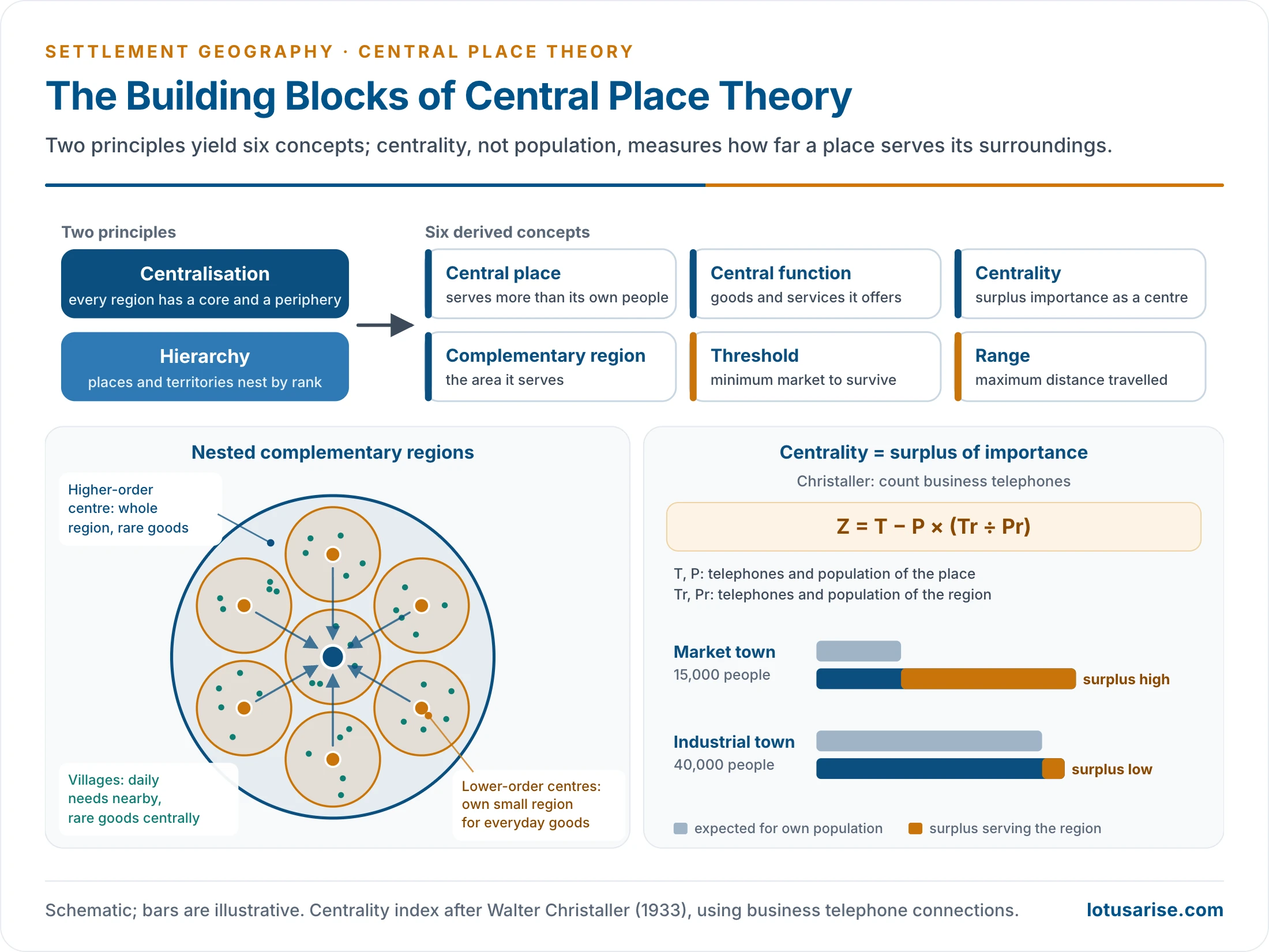
- Six derived concepts follow: central place, central function, centrality, complementary region, threshold and range.
Central Place
- A central place is a settlement that supplies goods and services to the population of surrounding settlements as well as its own.
- Every settlement that does this is a central place at its own level: a town for villages, a metropolis for towns, a capital for the metropolis region.
- It is a permanent settlement with maximum pull and many functions (trade, transport, health, education, administration). A periodic fair without permanent establishments is not one.
- Not every urban place is a central place. A mining or manufacturing town qualifies only if it also serves its surroundings.
- In the model the central place is a dimensionless point.
Central Functions
- Central functions are the goods and services a central place offers. A place offers several, of different orders.
- A district town has a civil court; Delhi adds the Supreme Court.
- Christaller grouped goods by where they are offered:
- Central goods and services, offered at central places: administration, banking, specialist hospitals, universities, airports.
- Dispersed goods, produced at scattered points: farm, forest and cottage products.
- Indifferent goods, found everywhere: basic utilities, petty roadside shops.
- He avoided the British habit of dividing goods into rural and urban. Using Alfred Weber’s terms, central goods may be consumer-oriented (bakeries, breweries) or raw-material-oriented (dairies, sugar mills).
Centrality
- Centrality is the relative importance of a place as a service centre. It depends on the number, variety and order of its central functions, not on its population or its location.
- Christaller defined it as the surplus of importance: services supplied beyond the needs of the place’s own residents.
- Places with a surplus are importance-surplus places. Small places that rely on others are importance-deficit places.
- He measured it with business telephone connections: centrality Z = T − P × (Tr ÷ Pr).
- T and P are the telephones and population of the place; Tr and Pr are those of the region. The second term is the number of telephones the place would have at the regional average.
Complementary Region
- The complementary region (Ergänzungsgebiet), also called the tributary, service or market area, is the area a central place serves and which supports it in return.
- Its extent depends on the functional order of the centre, not simply on its population.
- On an isotropic plain, distance decay acts equally in all directions, so the ideal complementary region is a circle around the place.
- Distance decay means that interaction between two places weakens as the distance between them grows. It bites hardest on higher-order functions.
- A large complementary region contains several smaller ones, because small centres depend on larger ones for higher-order goods. This gives a nested hierarchy of service areas. The largest centre becomes the regional capital, and the whole region is its complementary region.
- Regions of the same order are equal in size and lie side by side; centres of the same order are equidistant.
- Christaller’s complementary regions differ in two ways:
- By order: from the small region of a market hamlet to the region of a regional capital, each three times the one below in the marketing system.
- By principle: under marketing, centres on the region’s corners are shared by three regions; under transport, centres on its edges are shared by two; under administration, the region is self-contained, with every dependent centre inside it.
Threshold
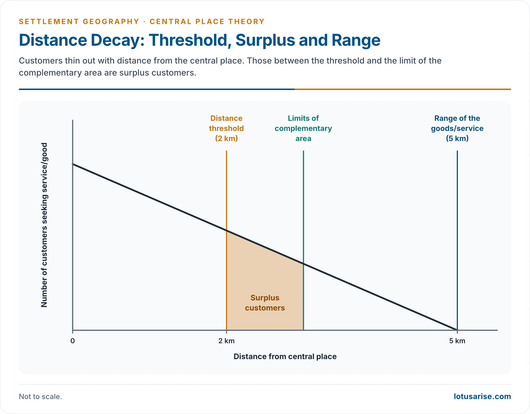
- The threshold is the minimum population or purchasing power needed to keep a function profitable. Below it the good cannot be supplied.
- Low-order goods (groceries, a primary school) have low thresholds and are bought often, from the nearest place.
- High-order goods (cars, specialist hospitals, universities, designer jewellery) have high thresholds. They are bought rarely and cluster in large cities.
- Hence grocery shops outnumber jewellers in every region.
- Rough scale of thresholds: a primary school needs one village, higher secondary education two or three villages, a university a city, and civil aviation a metro or large city.
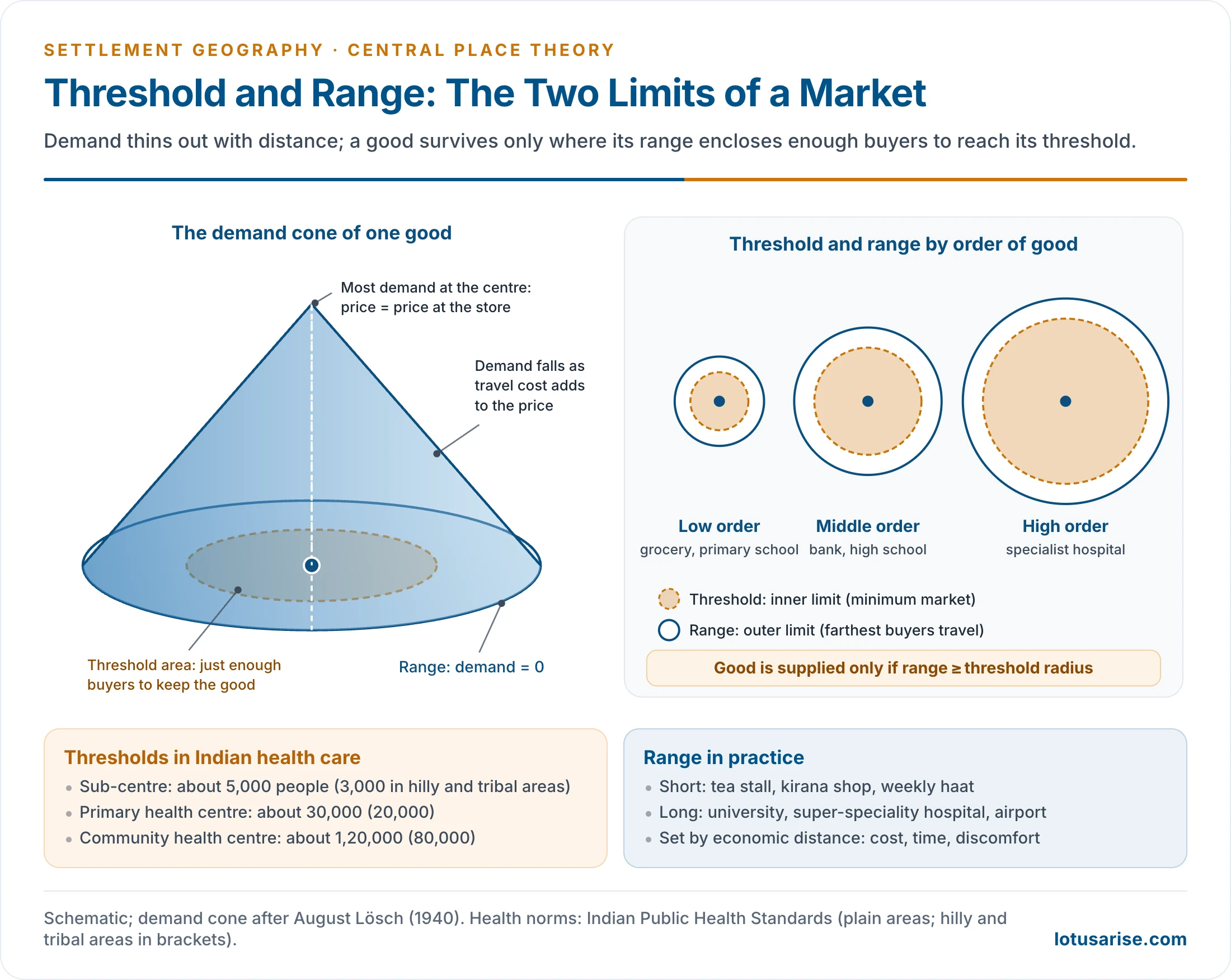
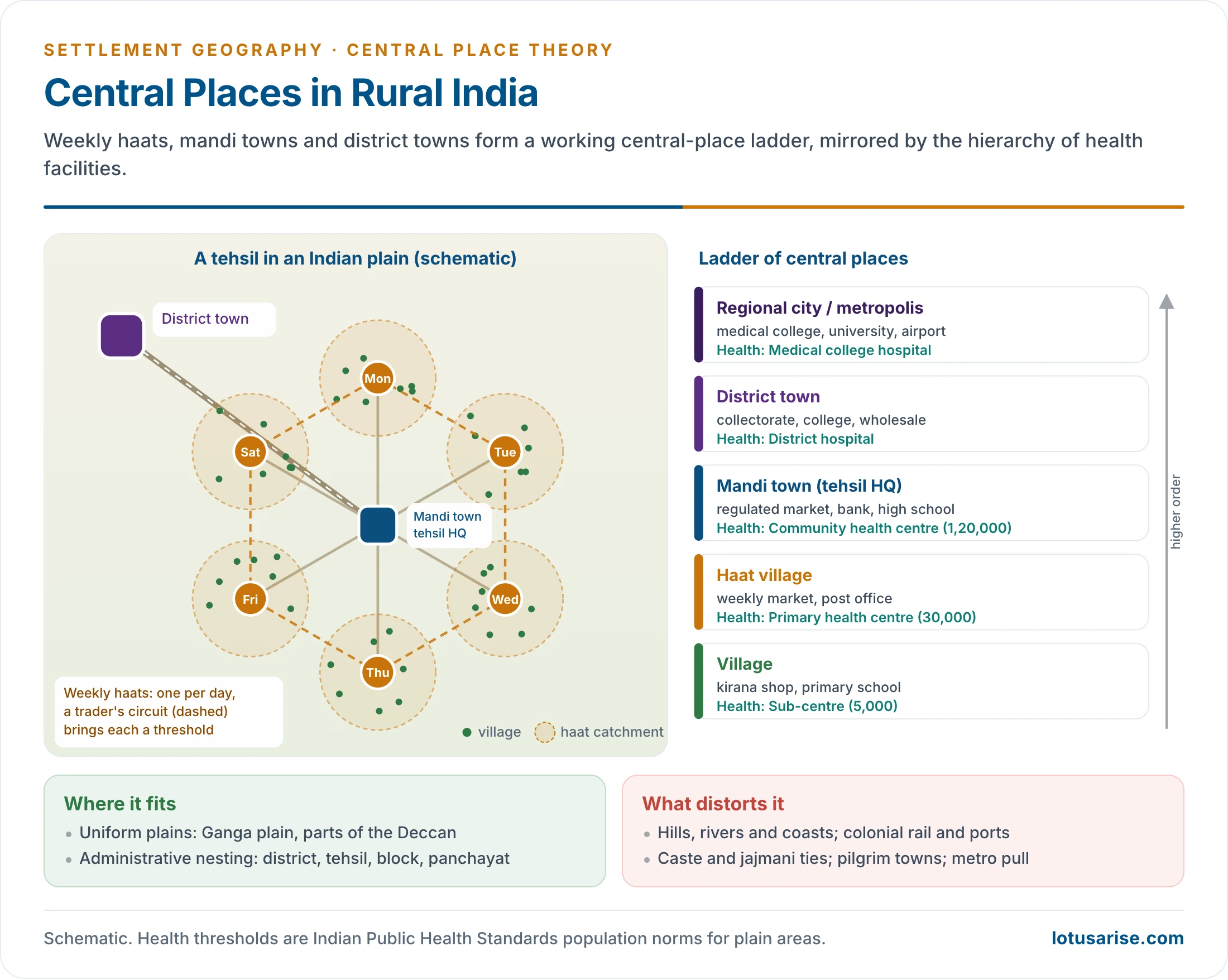
- India’s health network works on population thresholds (Indian Public Health Standards): a sub-centre for about 5,000 people, a primary health centre for about 30,000 and a community health centre for about 1,20,000 in the plains, with smaller norms in hilly and tribal areas.
Range
- The range is the maximum distance people will travel for a good. It is the outer limit of the market area. Beyond it, consumers go to another centre or do without.
- It measures economic distance: transport cost, travel time, discomfort, insurance, storage and spoilage, not kilometres alone.
- A tea stall or weekly market has a short range; specialist medical care and universities draw people from hundreds of kilometres.
- The range rises with the order of the good.
- Daily cases: a cold or cough goes to the primary health centre, a spinal injury to AIIMS; a costly car is bought in a metro. The Supreme Court at Delhi has the widest range and threshold of all.
- Threshold and range are properties of the goods and services offered, not of the place itself.
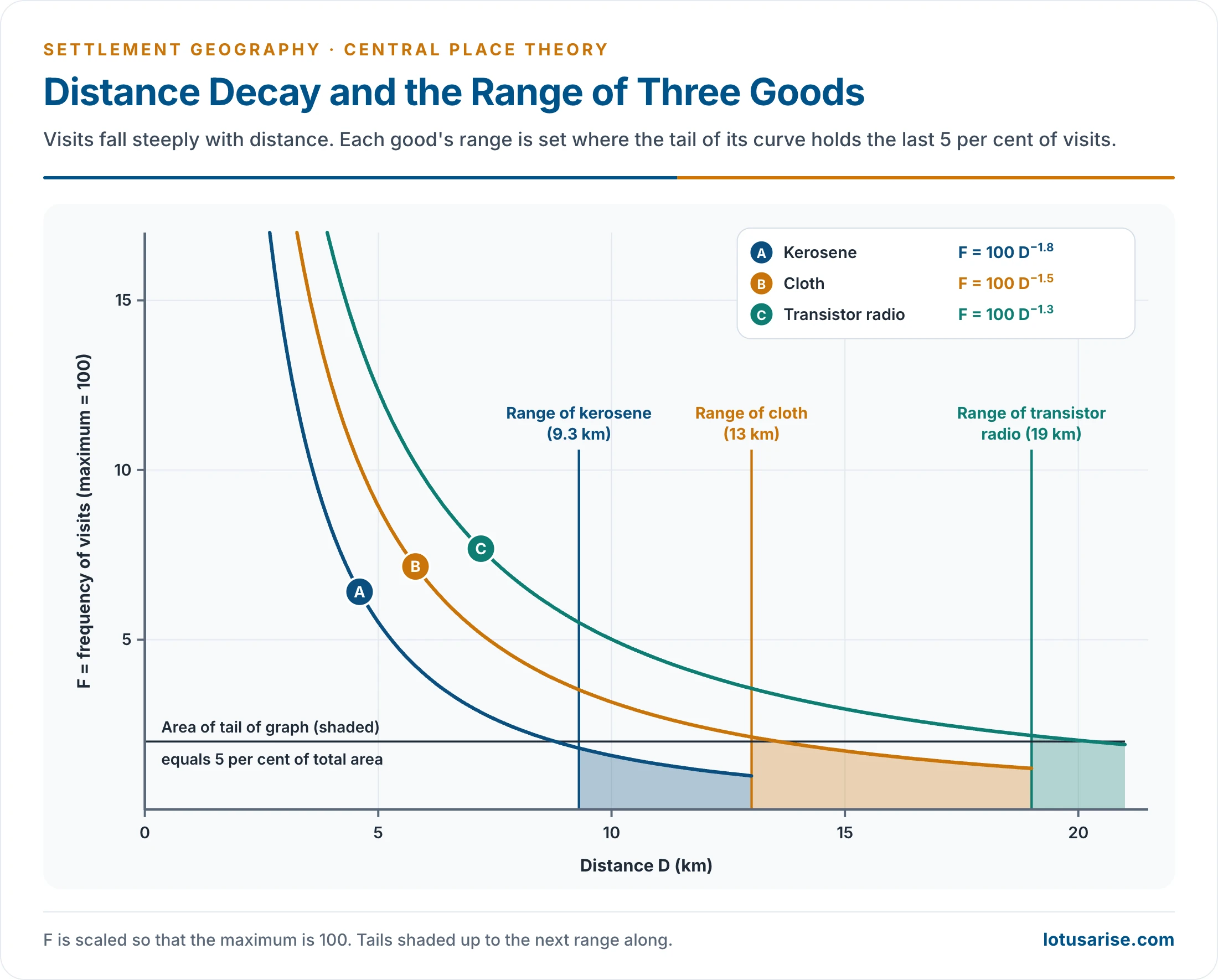
- Field curves show visits falling steeply with distance. On R. Ramachandran’s curves the ranges are about 9.3 km for kerosene, 13 km for cloth and 19 km for a transistor radio (F = 100 D^−1.8, 100 D^−1.5 and 100 D^−1.3, where F is visit frequency and D distance). The range is set where the tail of the curve holds the last 5% of visits.
- Where the threshold distance is 2 km and the range 5 km, the customers between the threshold and the limit of the complementary region are surplus customers.
- The threshold is the inner limit and the range the outer limit. A good can be supplied only where its range is at least the radius that encloses its threshold population.
- The ideal (upper) range is where demand falls to zero. The real range is often shorter, ending where a competing centre becomes cheaper to reach.
- If the range exceeds the threshold radius, the supplier earns excess profit, which draws in competitors until market areas shrink back towards the threshold.
From Circles to Hexagons
- For an ideal resolution of the settlement pattern:
- each complementary region holds exactly the threshold population;
- the range equals the radius of the region, since a shorter range would leave edge consumers unwilling to travel;
- a higher-order centre also offers every lower-order function: Delhi has parliamentary and judicial functions as well as railway stations and grocery shops.
- Buyers and sellers pull in opposite directions:
- Buyers want many centres, to cut travel.
- Sellers want few centres, to enlarge their markets.
- CPT seeks the number of centres at which neither side gains an advantage, a trade-off in the number of centres and of hierarchical levels.
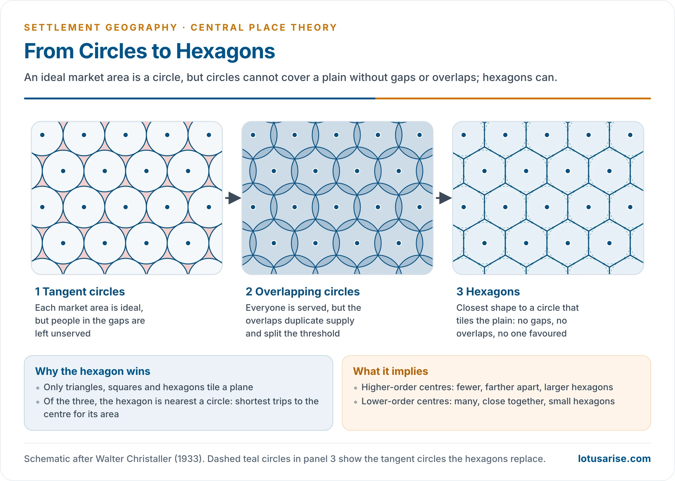
- Circles enclose the most area for a given perimeter, but:
- tangent circles leave unserved gaps;
- overlapping circles duplicate supply and split the threshold.
- The hexagon is the shape closest to a circle that fills the plane without gaps or overlaps. Christaller therefore used a hexagonal lattice of market areas, which favours neither buyer nor seller.
- In that lattice:
- higher-order centres are fewer and farther apart (Delhi, Mumbai, Chennai, Kolkata);
- lower-order centres are more numerous and closer together (towns and villages).
The Three K-Principles
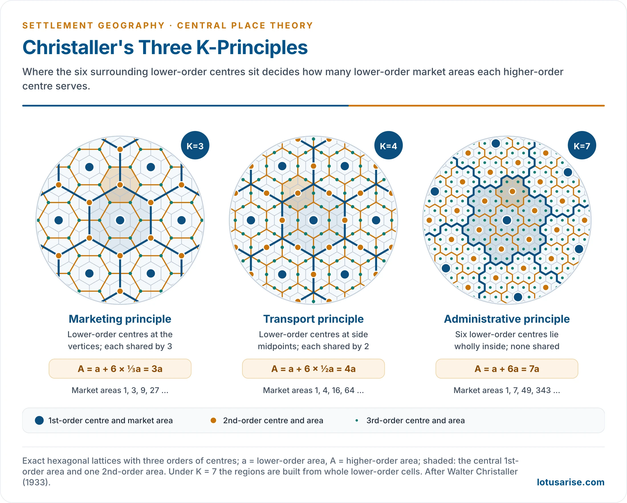
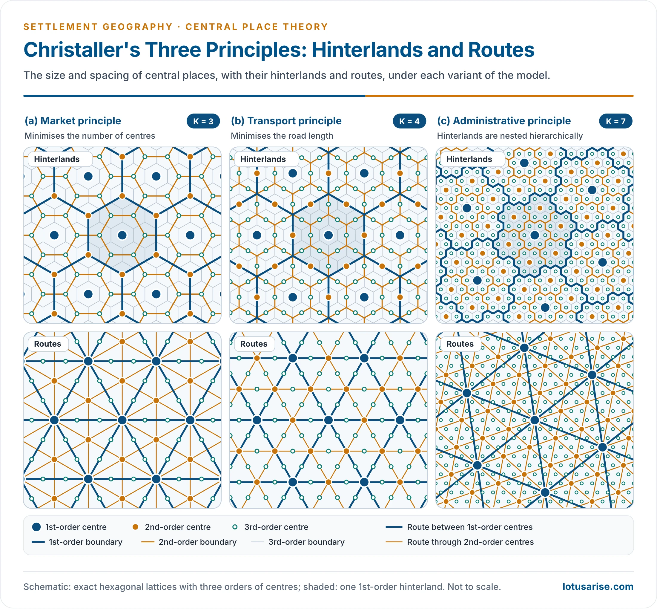
- Christaller derived three arrangements of centres, each from a different organising principle and each with its own K-value.
- K is the number of lower-order market areas served by a higher-order centre, counting its own. It is the constant ratio between the market areas of successive orders.
- In every arrangement a higher-order centre is ringed by six centres of the next lower order. What changes is where these six sit, and so how much of their market areas it serves.
- Read as a pyramid: one metropolis at the centre, six cities around it, many more towns around each city and still more villages around each town.
- Lower-order hexagons are nested within higher-order ones, a nested pattern of hierarchy. Christaller worked with seven orders in each system.
Marketing Principle (K = 3)
- Lower-order centres sit at the vertices of the higher-order hexagon. Each is shared by three higher-order centres.
- Every consumer is then as close as possible to a centre of each order, so the fewest centres serve the whole area.
- A higher-order centre serves its own area plus one-third of each of the six around it:
- A = a + 6 × ⅓a = 3a, so K = 3.
- Market areas grow as 1, 3, 9, 27, 81. Counting each centre at its highest order, the number of places per order is 1, 2, 6, 18, 54, 162.
- Spacing between centres grows by √3 at each step up.
- Christaller found it the main principle, typical of thinly settled agricultural areas.
Transport Principle (K = 4)
- Lower-order centres sit at the midpoints of the sides of the higher-order hexagon. Each is shared by two higher-order centres.
- As many centres as possible then lie on straight routes between higher-order centres, so road length and transport cost are least.
- A = a + 6 × ½a = 4a, so K = 4. Market areas grow as 1, 4, 16, 64, and spacing doubles at each step.
- Counting each centre at its highest order, the number of places per order is 1, 3, 12, 48, 192.
- The older colonial landscape organised by railways, including parts of British India, shows it best.
- It prevails where traffic routes dominate: busy corridors, valleys and densely settled transit regions.
Administrative Principle (K = 7)
- All six lower-order centres and their areas lie wholly within the higher-order area.
- No lower-order place is split between two higher-order centres, so there is no divided jurisdiction.
- A = a + 6a = 7a, so K = 7. Market areas grow as 1, 7, 49, 343.
- Counting each centre at its highest order, the number of places per order is 1, 6, 42, 294.
- The region’s outer lines pass midway between dependent settlements, so the tributary area is clearly marked.
- It suits centralised administration, political control and defence.
| Principle | Aim | Lower-order centres sit | Share of each served | K | Market areas by order |
|---|---|---|---|---|---|
| Marketing | Fewest centres, shortest trips | At hexagon vertices | One-third | 3 | 1, 3, 9, 27 |
| Transport | Most centres on straight routes | At side midpoints | One-half | 4 | 1, 4, 16, 64 |
| Administrative | No split jurisdictions | Wholly inside | Whole | 7 | 1, 7, 49, 343 |
- The three principles can work in one region at once: market functions on K = 3, transport on K = 4, administration on K = 7.
- This changes the size of market areas, not the order of functions. In southern Germany the marketing principle dominated; transport and administration produced local deviations.
- Christaller’s own tests: the marketing principle held in thinly settled farming areas such as Bavaria east of the Rhine and Lorraine; the transport principle along the Rhine plain and other busy corridors; the administrative principle where political borders split one expected centre into several, as at Basel, Freiburg and Mulhouse.
- India, with many organising logics side by side, shows the same mixing of principles.
- The principles cover marketing, transport and administration only. Manufacturing is left out, a gap Lösch later addressed.
The Hierarchy of Central Places in Southern Germany
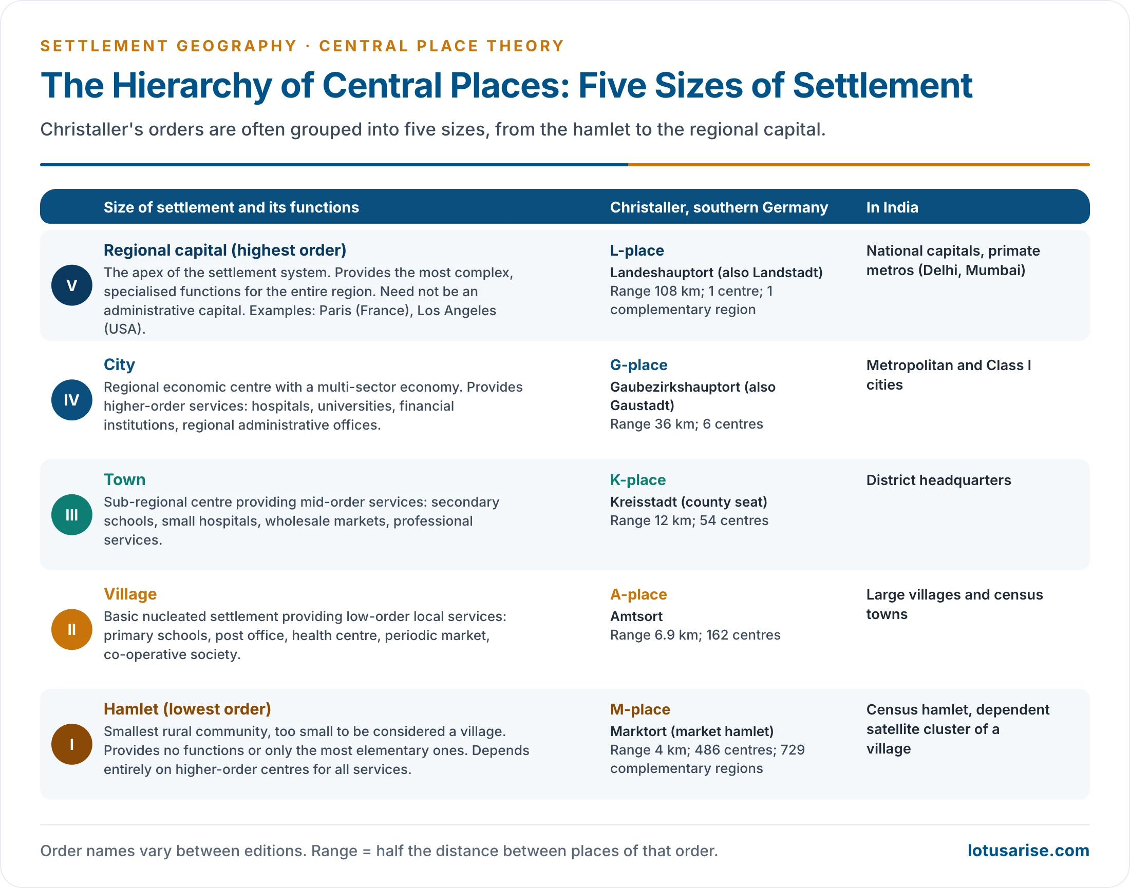
- Christaller recognised seven orders, from the market hamlet (Marktort) to the regional capital (Landeshauptort), with auxiliary places below them.
- Each order has all the functions of the orders below plus more specialised ones.
- Order names vary between editions: Bezirksstadt, Gaustadt, Provinzstadt and Landstadt also occur for B, G, P and L.
- Range of each order (half the distance apart): M 4, A 6.9, K 12, B 20.7, G 36, P 62.1 and L 108 km. Complementary regions served: 729, 243, 81, 27, 9, 3 and 1.
- The orders are often grouped into five sizes of settlement:
- Hamlet (M): too small to count as a village; few or no functions. In India, a census hamlet or a dependent cluster.
- Village (A): primary school, post office, health centre, periodic market, co-operative society. In India, large villages and census towns.
- Town (K): secondary schools, small hospitals, wholesale markets, professional services. In India, district headquarters.
- City (G): hospitals, universities, financial institutions, regional offices. In India, metropolitan and Class I cities.
- Regional capital (L): the most specialised functions for a whole region; it need not be an administrative capital (Paris, Los Angeles). In India, national capitals and primate metros such as Delhi and Mumbai.
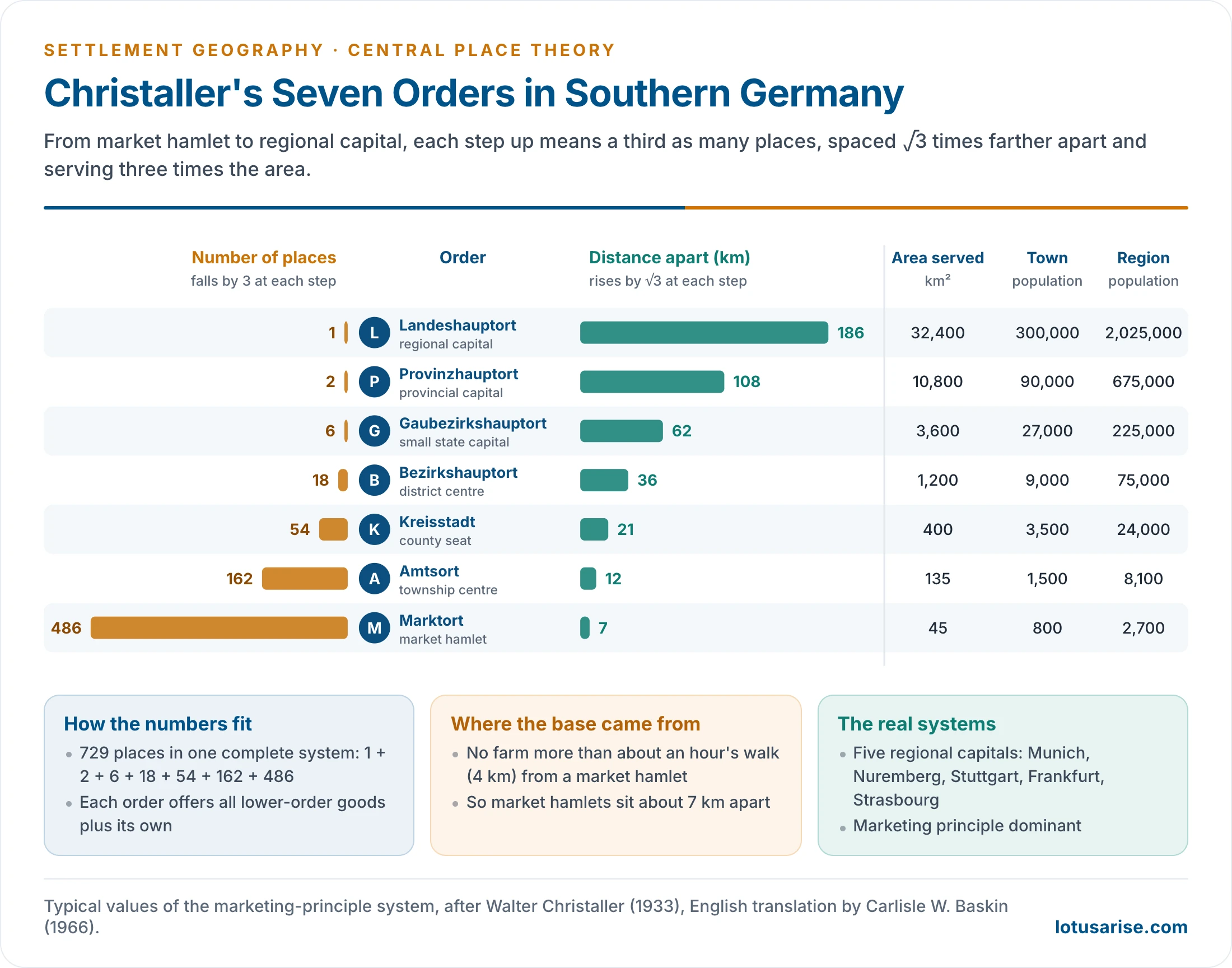
- Numbers fall by a factor of three and spacing widens by √3 at each step.
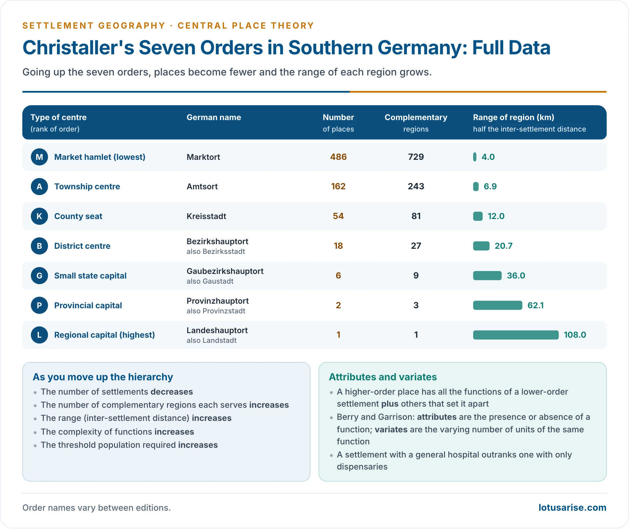
- Five regional capitals anchored the systems he mapped: Munich, Nuremberg, Stuttgart, Frankfurt and Strasbourg.
- In one complete L-system of the marketing principle there are 729 places: 1 L, 2 P, 6 G, 18 B, 54 K, 162 A and 486 M. The 729 market-hamlet regions are the smallest cells of the lattice.
- The base spacing came from walking distance: no farm should be more than about an hour’s walk (roughly 4 km) from a market hamlet, which puts market hamlets about 7 km apart.
| Order | Central place | Places | Distance apart (km) | Tributary area (km²) | Population of place | Population of region |
|---|---|---|---|---|---|---|
| M | Marktort (market hamlet) | 486 | 7 | 45 | 800 | 2,700 |
| A | Amtsort (township centre) | 162 | 12 | 135 | 1,500 | 8,100 |
| K | Kreisstadt (county seat) | 54 | 21 | 400 | 3,500 | 24,000 |
| B | Bezirkshauptort (district centre) | 18 | 36 | 1,200 | 9,000 | 75,000 |
| G | Gaubezirkshauptort (small state capital) | 6 | 62 | 3,600 | 27,000 | 225,000 |
| P | Provinzhauptort (provincial capital) | 2 | 108 | 10,800 | 90,000 | 675,000 |
| L | Landeshauptort (regional capital) | 1 | 186 | 32,400 | 300,000 | 2,025,000 |
Evaluation of Christaller’s Theory
Contributions
- The first general theory of settlement location, a pillar of the quantitative revolution and the base of later work on urban systems.
- It introduced threshold, range, centrality and hierarchy, still the working tools of retail, health and service planning.
- It shows that settlements are not arbitrarily located: trade and service provision put an order into their spacing.
- As a normative benchmark, it lets real patterns and their deviations be measured.
- It has guided planning:
- the new villages and towns of the Netherlands’ IJsselmeer polders (Noordoostpolder, Flevoland);
- Israel’s Lakhish region settlements of the 1950s;
- less happily, Nazi Germany’s resettlement plans for occupied Poland, on which Christaller himself worked.
- The hexagonal cells of mobile-phone networks use the same geometry.
Criticisms
- Unreal assumptions:
- Isotropic plains are rare. Mountains, rivers, coasts and deserts change routes and costs.
- Population and purchasing power are uneven, and so are resources.
- Consumers are satisficers, not optimisers. They make multipurpose trips, chase price and quality, and act from habit and loyalty.
- Perfect competition does not exist. Agglomeration economies, historical head starts and state decisions (new capitals, SEZs, Chandigarh) override market logic.
- Chandigarh shows the point: it became Punjab’s capital by political decision, after Lahore went to Pakistan.
- A settlement can have many functions, and its dominant function can change, as when a mining town becomes a service centre.
- Weak model structure:
- Static: it describes an equilibrium, not how the system grows with technology, income and population.
- It takes the hierarchy for granted. Christaller assumed a system of one large city, fewer towns and many villages already existed, and explained its spacing, not how some places came to outgrow others.
- Built for a pre-industrial farming landscape; it ignores manufacturing.
- Fixed K and strict nesting are rarely observed; empirical tests seldom find hexagons.
- Humanistic critique:
- It is normative, not descriptive: where centres should be, not where they are.
- It ignores perception, culture and social relations; universal market optimisation is a Western economic idea.
- Modern transport, telecommunication and e-commerce have shrunk distance.
- Where it fits best: large, developed, service-based economies with extensive plains, such as Germany, France and the farm belt of the USA. Germany’s spatial planning still assigns towns to tiers of higher-, middle- and basic-order central places (Ober-, Mittel- and Grundzentren) when locating public services.
- These are also the countries where the rank-size rule is found.
- Overall judgement:
- Normative models cannot claim universal applicability, but they are desirable, because they bring structure and scientific method to the subject.
- They are stochastic, half-true laws that reveal the ideal and the real together.
- Lösch’s changes mark Christaller’s main gaps: fixed K, a supply-side view, rigid nesting, simple geometry and the reduction of all goods to three principles.
Lösch’s Economic Landscape
Approach
- August Lösch published his model in Die räumliche Ordnung der Wirtschaft (1940; English translation The Economics of Location, 1954).
- He kept Christaller’s uniform plain, rational actors, threshold, range and hexagons.
- He was a moderate critic, since he accepted much of Christaller. His approach was more empirical and inductive, using urban places across Germany as well as Iowa.
- It was the first attempt at a general theory of location built on demand.
- Assumptions: a uniform plain with self-sufficient farms evenly spaced on a triangular lattice; identical tastes and incomes; transport cost proportional to distance; supply held constant while demand falls as price rises.
- Demand cone: the price a consumer pays rises with transport cost, so demand falls with distance from the producer, reaching zero at the range. Rotating this demand curve around the producer gives a cone, whose volume is total sales.
- Each good has its own threshold, range and hexagonal market area. Producers locate to command the largest revenue.
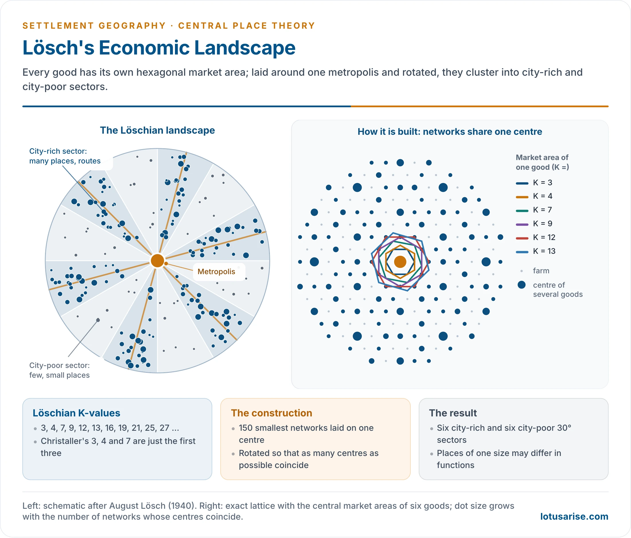
- Starting from evenly spread, self-sufficient farms, the market area of a good can enclose 3, 4, 7, 9, 12, 13, 16, 19, 21, 25, 27… settlements (the Löschian numbers).
- K varies freely from good to good. Christaller’s 3, 4 and 7 are only the three smallest cases.
Construction of the Landscape
- Lösch took the 150 smallest hexagonal networks, one for each size of market area, and laid them so that all share one centre, the metropolis.
- Older accounts describe this as 150 goods and services stacked with the highest order at the base, over some 40 networks, with rich and poor sectors marked by the cost of a commodity or service.
- He rotated the networks about that centre so that as many production centres as possible coincide. Where several coincide, a larger, multi-function place arises.
- The result is the Löschian economic landscape:
- a metropolis at the centre, with radial transport routes;
- twelve 30° sectors around it: six city-rich sectors, where centres coincide, alternating with six city-poor sectors;
- places of the same size need not have the same functions, so regions specialise and some goods are missing from parts of the landscape;
- city sizes form a continuous gradation rather than fixed steps, and orders interweave.
- Agglomeration drives the pattern. Firms cluster to share a labour market, customers and infrastructure (economies of scale), so centres are not uniform even on a uniform plain.
- Lösch checked his predicted spacing against the towns of Iowa (USA). The observed distances between towns at successive levels came close to his predicted values, roughly doubling at each step up.
- The landscape is denser and looks more random, without Christaller’s neat geometry. A metropolis with radial routes and interwoven settlements of many sizes, such as Delhi and its region, resembles it.
Merits and Criticism
- Merits:
- Variable K, thresholds and market areas bring the model closer to reality.
- It includes production and manufacturing, regional specialisation and contrasts between rich and poor sectors.
- A continuous size distribution matches observed city sizes better than fixed tiers.
- The most purchases can be made locally, with least total transport.
- Criticism:
- Still abstract and normative: the uniform plain and rational actors remain.
- Overemphasises demand and ignores the locational interdependence of firms and industries.
- Complicated: superimposed networks are hard to map and to follow. Lösch did not explain his rotation fully, and later geometric work (John U. Marshall, 1977) questioned whether city-rich and city-poor sectors arise at all.
- Its base of evenly spread farms fits only rural regions.
Christaller and Lösch Compared
| Basis | Christaller (1933) | Lösch (1940) |
|---|---|---|
| Discipline | Geographer: towns as service centres | Economist: general theory of location |
| Direction of build | Top-down, from the highest order | Bottom-up, from the smallest market areas |
| Driving force | Supply of services to a complementary area | Demand and profit; centres are also production sites |
| Economy modelled | Services (tertiary) | Includes manufacturing |
| K-value | Fixed: 3, 4 or 7 | Free: 3, 4, 7, 9, 12, 13… |
| Goods | Grouped under three principles | Each good its own network (150 networks) |
| Hierarchy | Fixed tiers, fixed numbers per tier (1, 2, 6, 18…) | No fixed tiers; orders interweave |
| Places of one size | Identical functions | Different functions; specialisation |
| Pattern | Uniform hexagonal lattice | City-rich and city-poor sectors round a metropolis |
| Regional disparity | Not shown | Shown by rich and poor sectors |
| City sizes | Stepped classes | Continuous gradation under one metropolis |
| Suits | Thinly peopled, fully developed service landscapes | Denser landscapes with uneven development |
| Study area | Southern Germany | Tested on Iowa, USA |
| Character | Idealistic, lower empirical validity | Closer to reality, higher empirical validity |
| City-size model | Closer to the rank-size rule | Closer to the primate city |
| Forces | Centrifugal | Centripetal |
| Development stage | Fully developed landscape; developed countries | Landscape still developing; developing countries |
| Direction of flow | From higher to lower levels | From lower to higher; the main centre arises by polarisation of economic activity |
Later Modifications
- Walter Isard (1956): population density rises towards a metropolis, so market areas shrink near the city and widen away from it. The hexagonal net is distorted rather than uniform.
- Brian J. L. Berry and William L. Garrison (1958) gave the theory its functional basis.
- They separated attributes (whether a function is present) from variates (how many units of it there are), so a settlement with a general hospital outranks one with only dispensaries.
- In Snohomish County, Washington, they ranked 33 centres by the central functions they offered and estimated a threshold population for each function.
- Centres fell into distinct orders (villages, towns, cities), each marked by a set of functions entering at a given threshold: a stepped hierarchy grounded in thresholds rather than geometry.
- Berry later extended the idea to the hierarchy of business centres within cities.
- Probabilistic and dynamic models: Richard Morrill (1963) simulated the growth of Sweden’s town system, and Michael Dacey (1966) treated central-place locations as a probability pattern.
- John B. Parr (1978) allowed different K-values at different levels of one system, a mixed hierarchy closer to observed patterns.
- Periodic markets: G. William Skinner (1964) showed that rural China’s markets meet on fixed days in rotation, so a mobile trader reaches a threshold that no single fixed market would.
Applicability and Relevance
Application in India
- What fits:
- Administrative hierarchy (K = 7). National capital, State and UT capitals, divisions, districts, sub-districts (tehsil, taluk or mandal), blocks and gram panchayats nest so that each unit lies wholly within one higher unit, as the administrative principle requires. The number of levels is close to Christaller’s seven, but the ratio between levels is far from a constant seven.
- Marketing principle at district level. In uniform plains such as the Ganga plain and parts of the Deccan, tehsil towns and market centres serving surrounding villages show partial conformity to K = 3.
- Tehsil towns send about one-third of their population to the district town for higher-order goods.
- Periodic markets (haats, shandies, painths) form the base of the rural central-place system. A weekly market rotates among villages so that traders reach a threshold no single village provides. Daily markets in mandi towns, regulated wholesale markets and district towns sit above them, the pattern Skinner described for China.
- Threshold in services: primary schools and sub-centres in villages; colleges, district hospitals and specialist care in towns and cities.
- Ranking of villages by services: a first order with a health sub-centre, post office, primary school and periodic market; a second with a dispensary, telephone office, high school and permanent market; a third with a hospital, telephone exchange, college and wholesale market.
- This ordering by medical, communication, educational and commercial facilities is Mondol’s (1988).
| Level | Units in India (2026) | Ratio to level above | K = 7 ideal |
|---|---|---|---|
| National capital | 1 | — | 1 |
| States and UTs | 36 | 36 | 7 |
| Districts | 784 | about 22 | 49 |
| Sub-districts | about 7,100 | about 9 | 343 |
| Gram panchayats | about 2.55 lakh | about 36 | 2,401 |
| Villages | about 6.78 lakh | about 2.7 | 16,807 |
- An older comparison set actual counts against the K = 7 series of new places at each level:
| Level | Actual (older count) | K = 7 series |
|---|---|---|
| National capital | 1 | 1 |
| State capitals | 28 | 6 |
| Divisional commissioners | 300 | 36 |
| District headquarters | 600 | 216 |
| Tehsil headquarters | 2,400 | 1,296 |
| Blocks | 7,000 | 7,776 |
| Village panchayats | 2.75 lakh | 46,656 |
- The fit is closest at block level, and poor above and below it.
- On the older counts a State had 15–20 districts on average, and India over 6 lakh villages.
- A claim once repeated, that the theory was used to choose Telangana’s capital, has no support: Telangana kept Hyderabad under the Andhra Pradesh Reorganisation Act, 2014.
- What does not fit:
- Physical diversity: no isotropic plain exists across the Himalaya, the Thar, the Deccan and the coastal plains.
- Colonial distortion: railways and ports were built for export and control, not to link villages to their nearest market towns.
- Nisith Ranjan Kar’s study of Calcutta (1960): only a faint pattern of central places around the city, not the southern German geometry. History from the end of the 17th century, early physiographic advantages, rapid industrial growth and declining agriculture around the city broke the normal grading of the hierarchy.
- Consumer behaviour: richer rural households bypass lower-order centres for higher-order ones. Multipurpose visits, price differences, social position and the mode of transport shape the choice.
- V. Prakash Rao and R. Ramachandran showed this in Muzaffarnagar district, Uttar Pradesh (1974).
- Caste and the jajmani system long supplied services through hereditary obligation, not market demand.
- Religious and pilgrimage centres (Varanasi, Tirupati, Haridwar; Mecca abroad) have national or global spheres of influence unrelated to market spacing.
- Metropolitan polarisation: at the top, primate cities and regional primacy break the expected steps.
- Digital services (e-commerce, telemedicine, online education) let small towns reach services once found only in large cities.
- Indian geographers’ assessments:
- Qazi Ahmad: not applicable, because India’s landscape is still developing and its physiographic and climatic diversity is too great.
- Ram Lochan Singh: partly applicable from the district down to the panchayat level, but not at the top, where metropolitan polarisation and regional primacy dominate.
- Rameshwar Prasad Misra: applicable only once the landscape is fully developed, economically and demographically.
- The Löschian landscape fits parts of India better, as in metropolitan regions with radial routes and sectoral concentration.
Planning Applications
- Growth centres: Indian regional planning designated service and growth centres for rural hinterlands on central-place lines, the core of growth pole and growth centre planning.
- The Miryalguda taluka study (1971) of the National Institute of Community Development ranked settlements by central functions and proposed a hierarchy of rural growth centres.
- Community development blocks and Panchayati Raj institutions use block headquarters as service centres for surrounding villages.
- Shyama Prasad Mukherji Rurban Mission (2016): 300 clusters of villages given urban amenities, creating new middle-order central places.
- Smart Cities Mission (2015): 100 cities developed as higher-order centres for their regions, to reduce dependence on the largest metros.
- Health and education: facilities are allotted to settlement levels by threshold, from sub-centres and primary schools to medical colleges and universities.
- Retail location: chains use threshold and range to choose towns and sites.
- Transport networks: the K = 4 logic places lower-order centres on routes between major cities.
- Gap analysis: planners locate missing central places in a region and designate new centres to fill them.
- Agricultural marketing: the spacing of regulated markets (mandis) and rural haats is planned around the distance farmers can carry produce, a range problem. Sparse market density in eastern and north-eastern India forces farmers to sell to middlemen at the farm gate.
Relevance in the Present Context
- Still relevant:
- Threshold and range still decide where hospitals, malls, bank branches, EV-charging points and quick-commerce dark stores go, by catchment population and travel time.
- India’s rural service hierarchy (periodic market, mandi town, district town) still works on central-place lines.
- Planning norms, such as the population standards for facilities in India’s URDPFI Guidelines (2014), are central-place thinking.
- Weakened:
- Cheap transport and digital services loosen the range constraint; consumers skip levels.
- Cities increasingly act as nodes in networks with horizontal, complementary links, not only as tiers in a nested hierarchy. Central flow theory (Peter J. Taylor and colleagues, 2010) was proposed to complement CPT for these city-to-city flows.
- World cities serve global rather than regional hinterlands.
- CPT’s geometry has dated, but its concepts endure in the hierarchy of urban settlements and the sphere of urban influence.
Previous Year Questions
1988Analyse Christaller’s Central Place Theory and the modifications introduced in it and examine its relevance in the present-day context.1992Write short note: Central place theory.2000Explain the basis and applicability of Christaller’s Central Place Theory. Bring out the recent modifications.2002Bring out the main points of difference between the central place theories of Christaller and Losch.2007Give an account of the functional bases of central place hierarchy.2011Critically examine the salient features of Central Place Theory propounded by Christaller and Losch.2013What are the basic postulates in the Central Place Model of Christaller?2016Give a critical account of Lösch’s theory of central places.2017Discuss the applicability of Christaller’s Central Place Theory.2021Examine the relevance of the Central Place Theory of Christaller in the present context.2023Explain with suitable diagrams A. Lösch’s model of the Theory of Location related to Central Places. Why has this been criticized?2024What is complementary region? With reference to hierarchy of settlements, describe the different types of complementary regions as proposed by Christaller.





Couldn’t Thank enough, this got to be the best notes for the optional. Thanks a lot.
Most Welcome. keep reading
How was your exam after reading these notes…?
Download Complete Notes Here – https://store.lotusarise.com/product/upsc-geography-optional-complete-notes-pdf/
Good content,but it’s problem 150 words not simulat this writtens in exam.hall
Thanks a lot.
thanks for your view
Explain how you did the last table with the CPT and Actual values of Administrative centers in India
National Capital 1 1
State Capital 28 8….
It will be 28 and 6, I have corrected the same. Keep reading.
Thank you for responding.
I have never came across a calculation in Central plave theory like this.
Usually we see √3 multiples for distance calculations
And multiples of 3 for no of population.
First time encountering multiples of 6, any reason?
Again Thank you
Hierarchical level 1,6,36,216, etc.
/ Good
Application table is wrong how 6 and it’s multiple instead of 7
Good explanation… Thanks a lot.
One of the mesmerizing notes of this headache topic….🙏🙏
Download Complete Notes Here – https://store.lotusarise.com/product/upsc-geography-optional-complete-notes-pdf/
In a point.. applicability to India…plz confirm …in a given example..is it Telangana or Andrapradesh..
Keep posting such type of beautiful content ❤️❤️ you are very helpful
Best geography optional notes ever seen
Download Complete Notes Here – https://store.lotusarise.com/product/upsc-geography-optional-complete-notes-pdf/