

- The functional classification of towns groups urban centres by the dominant economic activity they perform: manufacturing, trade, transport, administration, defence, education, religion, recreation and so on.
- It is regarded as the most meaningful basis for classifying settlements, because towns differ from one another most clearly in what they do.
- Function explains why a town exists, what role it plays in the regional and national economy and what it supplies to its hinterland. Size, site, form and age describe a town; function explains it.
Functional Classification: Concept

Meaning and Rationale
- Every town performs two kinds of work:
- Basic (city-forming) activities sell goods and services outside the town and bring money in, as a steel plant, a port or a university does.
- Non-basic (city-serving) activities meet the needs of the town’s own residents, such as local shops, schools and municipal services.
- A town’s functional character is set by its basic activities. This is why classification looks for activities in which a town employs more workers than an ordinary town.
- The minimum requirements idea, developed by Edward Ullman and Michael Dacey (1960), treats the smallest share of workers that every town of a given size needs in an activity as non-basic; anything above it is basic.
- Function shapes form. A steel town, a cantonment and a pilgrimage town differ in land use, street plan, social mix and even seasonal population.
- Robert E. Dickinson called functions the driving force of city life, shaping its growth and morphology. It is function rather than size that lets towns be compared.
- Function also places a town in the urban system. Specialised towns depend on wide markets, while higher-order central places serve their surrounding regions with many functions.
- Urban settlements offer the widest range of functions, so most schemes deal with towns and cities rather than villages.
- Function is built into the very definition of a town in India: a census town must have at least 75% of its male main workers in non-agricultural work, besides a population of 5,000 and a density of 400 per km², the core of the Census definition of urban.
Difficulties in Classifying by Function
- Most towns are multifunctional. Large cities combine administration, trade, industry and services, so a single label hides as much as it reveals.
- Complexity grows with size: the bigger the city, the harder it is to name one dominant function.
- Choice of criteria is subjective. The scholar decides which activities to count, which data to use and where to draw the line between “ordinary” and “specialised”.
- Data limits. Classification depends on census occupation or employment data, which differ between countries and change between censuses.
- Functions change over time. A mining town may decline, a fort town may become a market town, and a mill town may turn into a service centre. Any classification is a snapshot of one census year.
- Context matters. A function that is high-order in a developing country (a bank branch, a hospital) may be commonplace in a developed one. A scheme designed for American cities needs adapting before it can be applied to India.
Uses of Functional Classification
- Understanding the urban system. It shows how towns divide work among themselves: which serve as markets, which as factories, which as administrative or religious centres, and how far each depends on its sphere of influence.
- Explaining form and society. The functional type helps explain a town’s land use, migration pattern, sex ratio and seasonal rhythm. Industrial and port towns attract male migrants; educational and pilgrimage towns swell and shrink with the calendar.
- Regional planning. Planners use it to choose growth centres, to place new industry and services, and to identify vulnerable single-function towns that need diversification.
- Comparison over time. Repeating the same method on successive censuses reveals functional change, for example the shift of old mill towns towards services.
- Comparison across countries, provided the same categories and thresholds are used.
Methods of Functional Classification
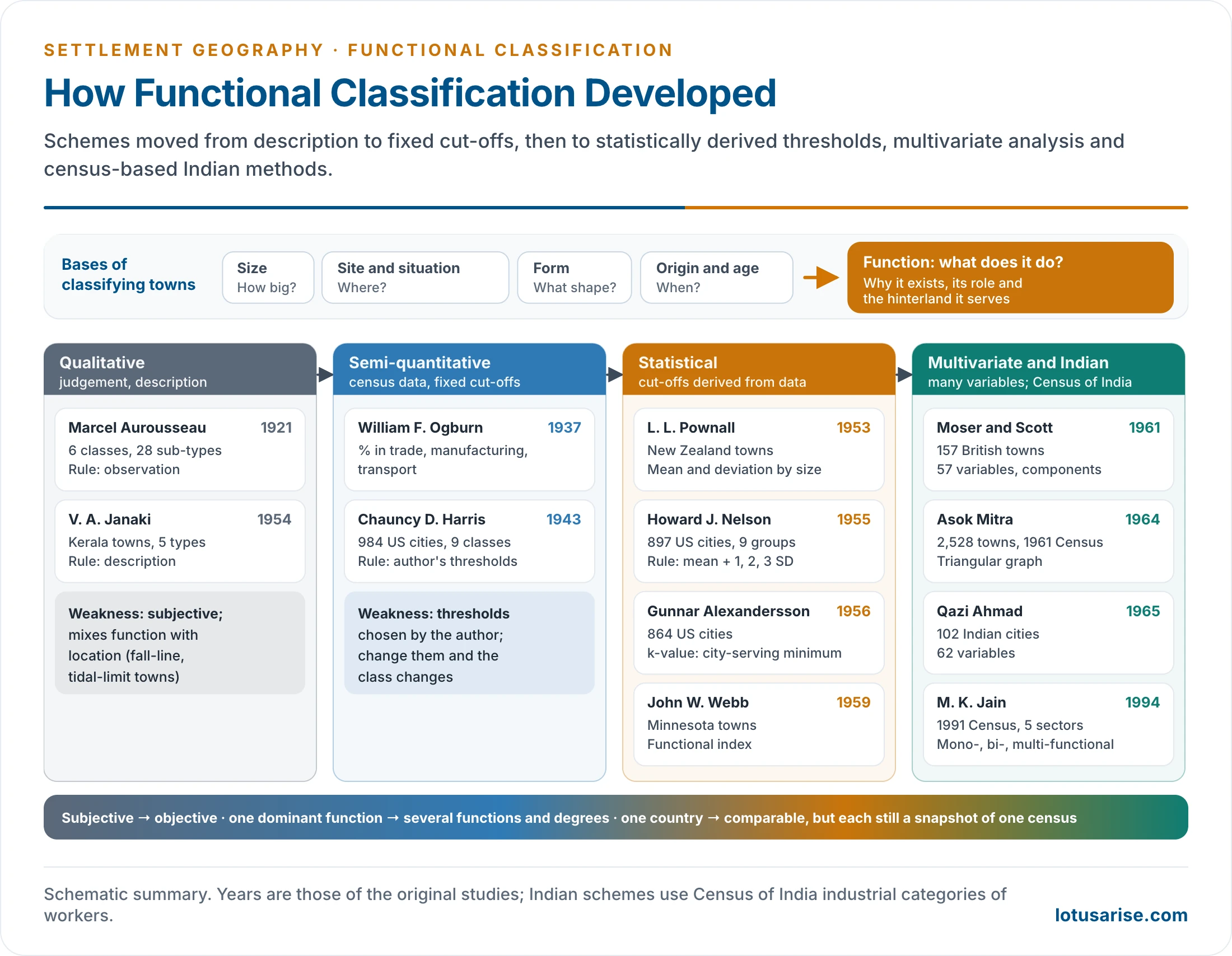
- Schemes have become steadily more statistical and more comprehensive since the 1920s. Three broad families are recognised, with a later fourth group of multivariate and Indian census-based methods.
| Family | Nature | Main scholars | Rule for “specialised” | Main weakness |
|---|---|---|---|---|
| Qualitative | Descriptive, empirical | Aurousseau (1921) | Observation and judgement | Subjective; mixes function and location |
| Qualitative-cum-quantitative | Census data, fixed cut-offs | Ogburn (1937), Harris (1943) | Percentages chosen by the author | Arbitrary thresholds |
| Quantitative (statistical) | Cut-offs derived from data | Pownall (1953), Nelson (1955), Alexandersson (1956), Webb (1959) | Mean, standard deviation, minimum requirement, indices | Snapshot; employment data only |
| Multivariate | Many variables at once | Moser and Scott (1961), Qazi Ahmad (1965), factor-cluster studies | Principal components, clusters | Complex; hard to interpret |
Qualitative Methods
- The earliest stage of functional analysis. Towns were classed by observation and description, without statistical criteria.
- These schemes gave later methods their vocabulary of town types.
- Other early schemes:
- R. D. McKenzie (1925): American communities as primary service, commercial, industrial and other.
- James: Indian towns as capitals, religious centres, army centres, markets, industrial towns and ports.
- V. Nath: eight economic categories of Indian towns.
Aurousseau’s Classification (1921)
- Marcel Aurousseau, in “The Distribution of Population: A Constructive Problem” (Geographical Review, 1921), produced the first systematic functional classification.
- He recognised six classes with 28 sub-types:
| Class | Sub-types |
|---|---|
| I. Administration | Capital cities, revenue towns |
| II. Defence | Fortress towns, garrison towns, naval bases |
| III. Culture | University, cathedral, art, pilgrimage and religious centres |
| IV. Production | Manufacturing towns |
| V. Communication | Collection (mining, fishing, forest, depot towns); transfer (market, fall-line, break-of-bulk, bridgehead, tidal-limit, navigation-head towns); distribution (export, import, supply towns) |
| VI. Recreation | Health resorts, tourist resorts, holiday resorts |
- Merits:
- The first comprehensive framework, a springboard for later methods.
- Simple and easy to apply.
- Covers cultural, recreational and defence roles that purely economic schemes miss.
- Criticisms:
- Over-generalised: six classes are too broad to separate cities.
- Subjective: no stated rule decides when a town belongs to a class; two scholars may class the same town differently.
- Time- and place-bound: fall-line and break-of-bulk towns belong to early 20th-century North America.
- Mixes function with location: “tidal-limit” and “fall-line” towns describe a site, not an activity.
- Ignores employment data altogether.
Qualitative-cum-Quantitative Methods
- A transitional stage. These schemes use census occupation and employment figures, but the qualifying percentages are chosen by the author.
Ogburn’s Classification (1937)
- William Fielding Ogburn classed American cities by the percentage of population engaged in trade, manufacturing and transport.
- It was one of the first uses of quantitative data, but the cut-off percentages were not derived from any statistical test.
Harris’s Classification (1943)
- Chauncy D. Harris, in “A Functional Classification of Cities in the United States” (Geographical Review, 1943), gave the most widely used scheme of this family.
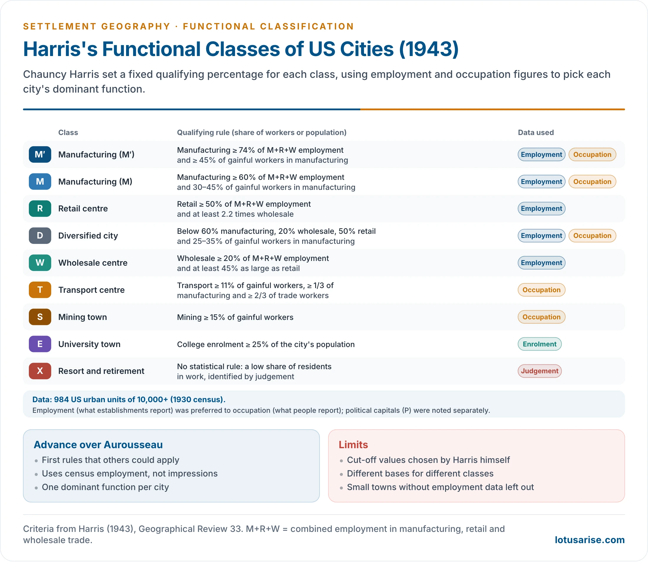
- Data: 984 US urban units of 10,000 or more people, using 1930 census figures.
- He used two sets of information: occupation figures (what people report they do) and employment figures (what establishments report they employ).
- He preferred employment figures, so that workers such as carpenters or plumbers working outside factories were not counted as manufacturing.
- Method: each city was assigned to the one activity of greatest importance, judged against fixed qualifying percentages.
- Nine principal classes: two manufacturing sub-types (M′ and M), retail (R), diversified (D), wholesale (W), transport (T), mining (S), university (E) and resort and retirement (X). Political capitals and other special towns (P) were noted separately.
- Key criteria:
- Manufacturing (M′): manufacturing is at least 74% of combined employment in manufacturing, retail and wholesale (M+R+W).
- Retail (R): retail is at least 50% of M+R+W employment and at least 2.2 times wholesale.
- Diversified (D): manufacturing below 60%, wholesale below 20% and retail below 50% of M+R+W.
- Transport (T): transport and communication employ at least 11% of gainful workers.
- Mining (S): at least 15% of gainful workers in mining.
- University (E): college enrolment equal to at least 25% of the population.
- Spatial pattern found by Harris:
- Manufacturing cities concentrated in the north-eastern Manufacturing Belt, where power, labour and markets were available.
- Retail and wholesale centres were spread through the agricultural interior, as central places serving their regions.
- Mining and resort towns were tied to resources and climate.
- Criticism:
- The scheme is subjective: the cut-off points were set by Harris’s own judgement, not by any statistical rule.
- Harold Carter (1975) made this objection.
- Different bases were used for different classes (employment for trade, occupation for transport and mining, enrolment for universities).
- Resort and retirement towns had no statistical criterion at all.
- Some choices were arbitrary; telephone and telegraph workers, for example, were left out of transport and communication.
- Harris used metropolitan districts as units, so smaller towns without such data were left unclassified.
- It gives one dominant function per city and says nothing about the degree of specialisation.
- The scheme is subjective: the cut-off points were set by Harris’s own judgement, not by any statistical rule.
- The method was followed, with changes, by Grace Kneedler Ohlson (1945), Victor Jones (1954) and John Fraser Hart (1955).
Quantitative (Statistical) Methods
- In statistical methods the threshold of specialisation is derived from the data, so the result is objective, transparent and repeatable.
- They rest on the idea of a diagnostic ratio: the share of the labour force in a function above which that function becomes distinctive compared with other towns.
- An early form was the location quotient of the British Political and Economic Planning report (1939): the share employed in a function in the town, divided by average employment in that function, × 100. A town at 100 is average; 110–129 is least specialised, 130–149 specialised, 150–169 highly specialised and 170 or more most specialised. It does not allow comparison within a town.
Pownall’s Classification (1953)
- L. L. Pownall classified the towns of New Zealand, comparing each town’s workforce with the mean and deviation of towns of its own size group.
- He recognised six functional groups: manufacturing; building and construction; primary industry; transport and communication; distribution and finance; and personal services.
- He measured each town’s positive deviation from the mean, so a town could specialise in more than one function. Older accounts count seven functions, splitting services into financial, hotel and personal, and administrative and professional, with a residential class from the ratio of earners to population.
Nelson’s Classification (1955)
- Howard J. Nelson published “A Service Classification of American Cities” in Economic Geography (1955). He removed the main weakness of earlier schemes by using a stated statistical procedure that others could check.
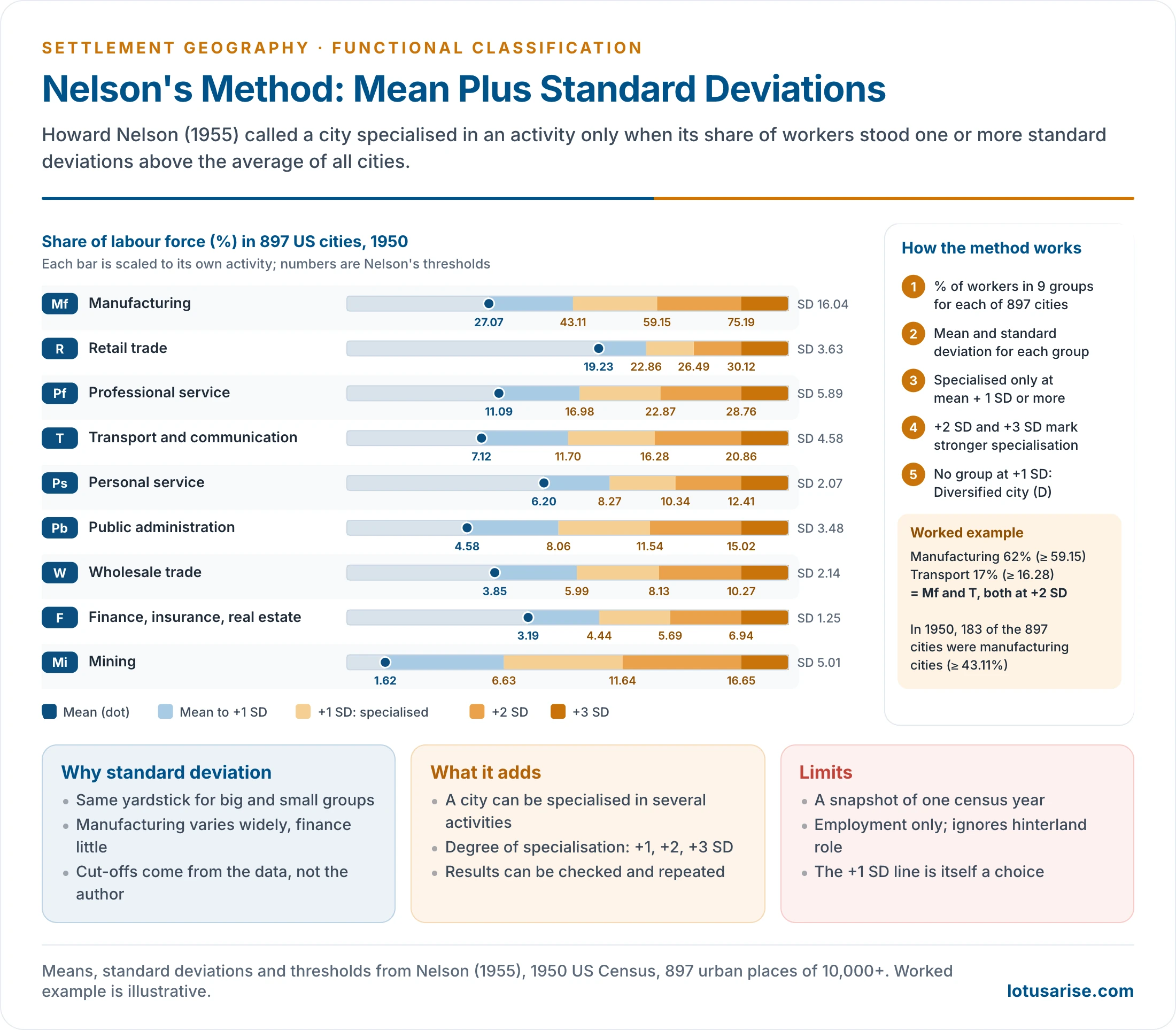
- Data: the 1950 Census of Population, for 897 urban places of 10,000 or more people.
- He grouped 24 industry groups into nine activity groups.
- He left out agriculture and construction, which were of little significance as urban functions.
- Nine activity groups: manufacturing (Mf), retail trade (R), professional service (Pf), transport and communication (T), personal service (Ps), public administration (Pb), wholesale trade (W), finance, insurance and real estate (F), and mining (Mi).
- Method:
- Calculate the percentage of workers in each activity group for every city.
- Find the arithmetic mean for each group across all 897 cities. Means ranged from 1.62% (mining) to 27.07% (manufacturing).
- Find the standard deviation (SD) of each group, a measure of how widely cities vary around the mean: SD = √(Σd² ÷ N), where d is a city’s deviation from the mean and N the number of cities.
- A city is specialised in an activity only when its share is at least mean + 1 SD. Shares of +2 SD and +3 SD mark stronger specialisation.
- A city that reaches +1 SD in no activity is classed as diversified (D).
- Ratings are written Mf1, Mf2 and Mf3 for +1, +2 and +3 SD in manufacturing, and so on. Washington D.C., with 31.6% in public administration, is the standard case of a very high rating.
- Example: the mean for manufacturing was 27.07% with an SD of 16.04%. A city needed at least 43.11% of its workers in manufacturing to qualify; 183 of the 897 cities did.
- Why the standard deviation: it is the simplest and best-known measure of variation, and it compares activities that employ large numbers (manufacturing) with those that employ few (mining, wholesale) on the same yardstick.
- Pattern: manufacturing was the most common specialisation, held by over a fifth of the cities and concentrated in the traditional manufacturing belt; retail specialisation was commonest in the central agricultural states.
- Contributions:
- A city can be specialised in more than one activity, and to different degrees.
- Nelson showed both a functional classification and a functional hierarchy for each activity.
- The shares employed in some activities vary with city size, a pattern he tested by size group.
- Criticism:
- Like any census-based scheme, it is valid for one point in time; occupation statistics change, while the long-built character of a town does not change as fast.
- British geographers, especially Claus A. Moser and Wolf Scott, raised this objection.
- The choice of +1 SD as the line of specialisation is itself arbitrary.
- It uses employment only. It ignores the town’s role for its hinterland, its institutions and its morphology.
- The SD assumes a roughly normal spread of values, which skewed activities such as mining do not show.
- Like any census-based scheme, it is valid for one point in time; occupation statistics change, while the long-built character of a town does not change as fast.
Alexandersson and Webb
- Gunnar Alexandersson (1956) studied 864 US cities and separated city-serving from city-forming employment.
- Mattila and Thompson (1955) had already used an index of surplus workers over the national or regional average.
- For each industry he took the share at which 5% of cities fall below (the k-value) as the minimum every city needs for itself.
- Employment above the k-value is city-forming and defines the town’s function.
- John W. Webb (1959), working on small towns of Minnesota, proposed a functional index and a specialisation index.
- Each function’s share in a town is weighted against its share in all towns, so that a town’s relative importance in each function can be measured and compared.
- Functional index FI = P ÷ Mp, where P is the percentage employed in a function and Mp its mean across towns. Specialisation index SI = sum of the functional indices ÷ 100. An SI of 1.00 means average employment; he set seven categories at 1.10, 1.20, 1.40, 1.80, 2.60, 4.20 and above.
Multivariate Methods
- From the 1960s geographers used many variables at once: employment, population, housing and social data.
- Claus A. Moser and Wolf Scott (1961) analysed 157 British towns on 57 variables and reduced them, by principal components, to a few underlying factors before grouping the towns.
- These methods give richer, multidimensional types but are computationally heavy and harder to interpret than a simple label.
Functional Types of Towns
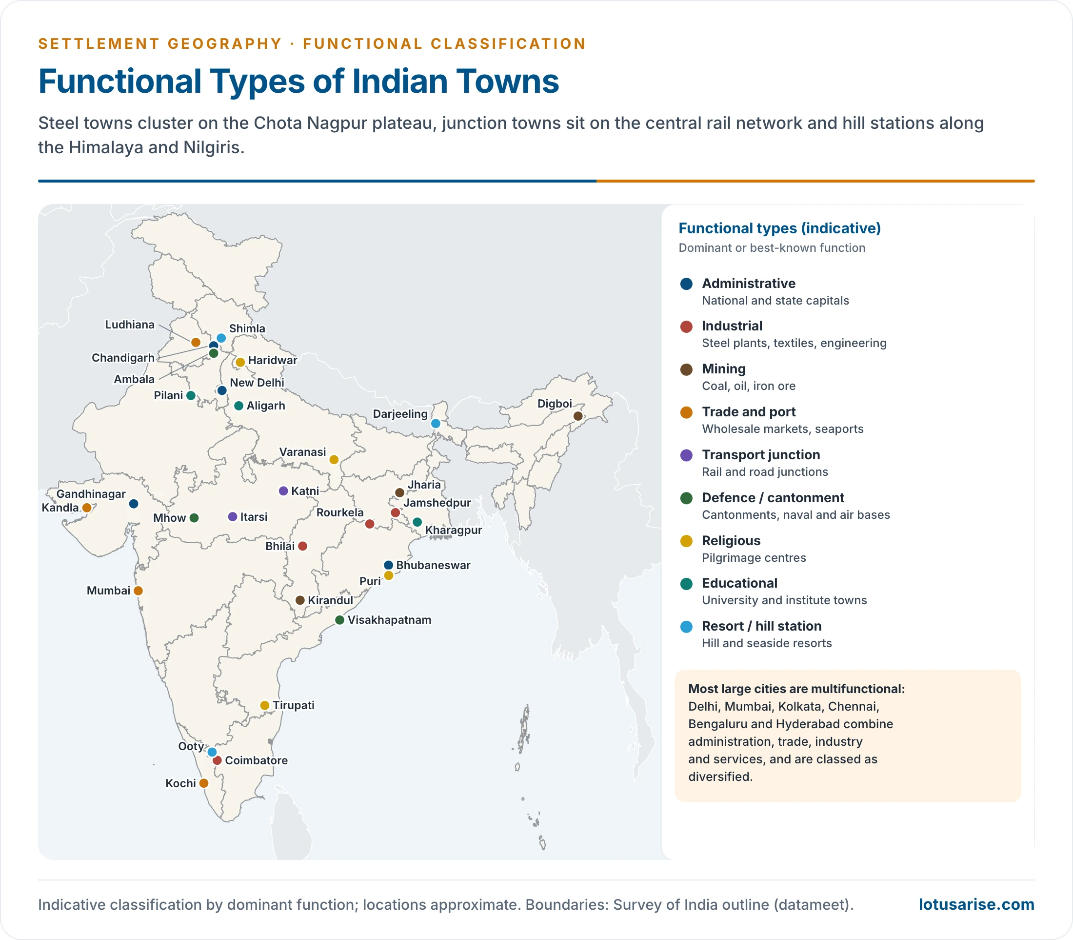
- Classification schemes, Indian and foreign, keep returning to a common set of functional types. Each type has a distinctive economic base, land use and location.
| Type | Dominant activity and character | Indian examples | World examples |
|---|---|---|---|
| Administrative | Government offices, legislatures, courts; employment tied to government | New Delhi, Chandigarh, Gandhinagar, Bhubaneswar, Jaipur, Bhopal, Patna, Lucknow, Aizawl, Kohima | Washington D.C., Canberra, Brasília, London, Moscow, Cairo, Tokyo |
| Defence | Cantonments, garrisons, naval and air bases at strategic sites | Ambala, Mhow, Pathankot, Udhampur, Visakhapatnam, Meerut, Jodhpur, Port Blair, Pune Cantonment, Adampur, Halwara, Jalandhar, Jamnagar, Khadakwasla | Gibraltar, Aden, Portsmouth, San Diego |
| Cultural: religious | Pilgrimage; temples, ghats, shrines; seasonal crowds | Varanasi, Haridwar, Tirupati, Puri, Amritsar, Ajmer, Dwarka, Madurai, Bodh Gaya, Prayagraj, Dharamshala, Gangotri, Pushkar | Mecca, Jerusalem, Vatican City |
| Cultural: educational | Universities and institutes; population falls in vacations | Aligarh, Santiniketan, Pilani, Kharagpur, Manipal, Amravati, Roorkee | Oxford, Cambridge, Harvard |
| Cultural: entertainment | Theatres, art galleries, film making | Mumbai, Chennai, Kolkata | |
| Collection (mining, fishing, forest) | Extraction of resources; boom-and-bust | Mining: Jharia, Raniganj, Digboi, Ankleshwar, Kolar, Kirandul (Bailadila), Zawar. Lumbering: Kathgodam, Haldwani, Kotdwar. Fishing: Machilipatnam, Kakinada, Mahe, Kozhikode | Kalgoorlie, Johannesburg (origin), Kirkuk, Hunan, Shanxi |
| Production (industrial) | Manufacturing; rail-linked to raw materials and markets | Jamshedpur, Bhilai, Rourkela, Bokaro, Durgapur, Coimbatore, Asansol, Bhadravati, Dhanbad, Visakhapatnam | Pittsburgh, Detroit, Magnitogorsk, Chicago, Glasgow, Shanghai, Manchester |
| Transfer and distribution | Trade, wholesale markets (mandis), warehousing | Ludhiana, Kanpur, Indore, Hapur, Mumbai, Kolkata, Chennai, Ahmedabad, Gwalior, Muzaffarpur, Surat, Bhopal | Kumasi, Alexandria |
| Transport | Rail and road junctions; break-of-bulk points | Itarsi, Katni, Mughalsarai, Kalka, Nagpur (highways converge) | Chicago (rail hub), San Francisco, Paris, Berlin, Santiago, Sydney |
| Seaport | Export and import; port industries | Kandla, Paradip, Haldia, Kochi, Tuticorin, Diamond Harbour, New Mangalore | Rotterdam, Shanghai, New York, Amsterdam, Cape Town |
| Resort and recreation | Hill stations, beaches, spas, heritage | Shimla, Darjeeling, Ooty, Mount Abu, Goa, Srinagar, Pahalgam, Gulmarg, Manali, Kullu, Dalhousie, Dharamshala, Nainital, Ranikhet, Pachmarhi, Dehradun, Agra, Jaipur | Venice, Las Vegas, Geneva, Los Angeles, Barcelona |
| Residential | Dormitory towns housing commuters | Noida, Navi Mumbai, Panchkula, Mohali, Rohini, Indirapuram | Levittown, Milton Keynes |
| Diversified | No single dominant function | Delhi, Mumbai, Kolkata, Chennai, Bengaluru, Hyderabad, Lucknow, Jaipur, Prayagraj | New York, London, Chicago, Kansas City |
Features of the Main Types
Administrative Towns
- Headquarters from which a country, state, district or sub-division is governed. They house legislatures, secretariats, courts and the residences of officials.
- The economic base depends heavily on government employment, which supports a large service and construction sector.
- Some are old capitals that grew naturally (Lucknow, Patna, Hyderabad). Others are planned capitals built for the purpose: New Delhi, Chandigarh, Bhubaneswar, Gandhinagar, Naya Raipur and Amaravati.
Defence Towns
- Built for the security of the state, usually at strategic sites: borders, passes, coasts and high ground.
- Older fort towns arose from Mughal and Rajput castles: Chittaurgarh, Ajmer, Jodhpur, Ranthambhore, Gwalior, Chanderi. Garh in a name usually marks a fort.
- Marked by cantonments, barracks, airfields, training areas, ordnance factories and naval dockyards.
- Land is clearly divided between military and civil authorities. The cantonment usually lies at a distance from, or at a corner of, the main town, a legacy of colonial planning.
Cultural Towns
- Religious towns grow at holy sites and pilgrimage centres. Temples, mosques, gurudwaras, ghats and dharamshalas dominate the core, and a pilgrimage economy (lodging, transport, ritual goods) supports the town. Crowds peak at fairs and festivals, as at the Kumbh in Prayagraj.
- Educational towns are built around universities and institutes. Bookshops, hostels and student services fill the town, and the population falls sharply in vacations, a diagnostic feature. Newer coaching hubs such as Kota show the same dependence on one sector.
Collection, Production and Trade Towns
- Collection towns (mining, fishing, lumbering) lie near the resource. They are the most vulnerable type: when the resource is exhausted or demand falls, they face decline and out-migration, as Kolar Gold Fields did after its mines closed in 2001.
- Production (industrial) towns have manufacturing as the main base.
- The scale and type of industry set the size and layout of the town; steel towns such as Jamshedpur, Bhilai and Bokaro were planned around the plant, with township housing for workers.
- They are well linked by rail and road for raw materials and markets.
- Transfer and distribution towns collect and distribute goods. Wholesale mandis, warehouses, cold stores and transport depots dominate. Market towns serve their rural hinterland; financial centres (Mumbai) handle banking, insurance and stock markets.
Transport Towns and Seaports
- Transport towns grow where routes converge or where one mode meets another.
- Railheads at the foot of the hills: Kalka, Kathgodam, Kotdwar.
- Junctions on trunk railway lines: Itarsi, Katni, Mughalsarai.
- Their economy is sustained by the traffic of people and goods passing through.
- Seaports link land and sea routes. Some serve as entrepôts, re-exporting goods from large warehouses, and many attract port-based industry such as refining at Haldia and Paradip and fertiliser and salt at Kandla.
Resort and Residential Towns
- Resort towns cater for recreation: hill stations (Shimla, Darjeeling, Ooty), seaside resorts (Goa), spas, heritage cities (Agra) and gateways to national parks. Hotels, shops and seasonal workers dominate, and many now face overcrowding, water shortage and waste problems in the tourist season.
- Residential (dormitory) towns grow around metropolitan cities as satellite towns. Most residents commute to the parent city; many, such as Gurugram and Noida, later acquire offices and industry of their own.
Diversified and Mono-functional Towns
- Diversified towns are the commonest type among large cities. Harris and Nelson both needed a “diversified” class for cities with no single dominant function.
- The Indian urban system is above all a system of diversified towns: capitals are also commercial, industrial and cultural centres, and seaports are also trading and service centres.
- Mono-functional towns carry a special risk:
- Dependence on one plant, one mine or one market exposes them to closure, price shocks, technological change and resource exhaustion.
- Their labour force is narrow in skills, and local government revenue depends on one employer.
- Examples: coal towns of the Jharia field facing fires and relocation, older single-industry mill towns, and tourist towns hit by the COVID-19 shutdown of 2020.
- Remedies: diversifying the economic base (services, small industry, education), skill training, better connectivity, and planning for the period after closure.
- Towns are also classed by age and cultural history (ancient, medieval, colonial, industrial and planned towns) and by stages of growth; these schemes belong to the wider classification of urban settlements and to the morphology of Indian cities.
- Cultural history: ancient, medieval, colonial, industrial-age and planned post-Independence cities.
- Griffith Taylor (1949): sub-infantile, infantile, juvenile, adolescent, early mature and mature towns.
- Lewis Mumford (1938): eopolis, polis and metropolis in growth; megalopolis, tyrannopolis and nekropolis in decay. His techno-economic phases are eotechnic, paleotechnic, neotechnic and biotechnic.
- Robert Redfield (1954): orthogenetic cities grow from indigenous culture; heterogenetic cities are shaped from outside.
Functional Classification of Indian Cities
The Indian Context
- Schemes built for American or European cities cannot be applied to India without change:
- Primary activities are significant in Indian towns. Many small towns have a large share of cultivators, agricultural labourers, fishers or plantation workers.
- Almost a third of urban centres have agriculture as a relatively dominant activity, and so do at least a quarter of census towns.
- Agricultural employment matters mainly in small towns. In large cities secondary and tertiary activities dominate.
- The towns range in size from under 5,000 to over ten million people and have long, layered histories.
- Function data are not standardised, for want of a single urban agency, so schemes differ between States and authors.
- Primary activities are significant in Indian towns. Many small towns have a large share of cultivators, agricultural labourers, fishers or plantation workers.
- All Indian schemes rest on the occupational data of the Census of India, which grouped workers into nine industrial categories in 1961–1991.
- 1961 categories: I cultivators; II agricultural labourers; III mining, quarrying, livestock, forestry, fishing, hunting and plantations; IV household industry; V other manufacturing; VI construction; VII trade and commerce; VIII transport, storage and communication; IX other services.
- From 1971 to 1991, mining and quarrying became category IV and household industry moved into category V.
Early Indian Studies
| Scholar | Year | Method | Scope and finding |
|---|---|---|---|
| V. A. Janaki | 1954 | Descriptive | Kerala towns in five types: administrative, commercial-industrial, trade (collection and distribution of farm produce), religious, plantation |
| Amrit Lal | 1959 | Location quotient | 67 Class I cities of the 1951 Census; most found multifunctional |
| Kashi Nath Singh | 1959 | After Nelson | Towns of Uttar Pradesh; many left unclassified |
| V. L. S. Prakasa Rao | 1960s | Least-squares regression of a function’s share on town size | Line of central value marks specialisation |
| S. M. Rafiullah | 1965 | Maximum positive deviation (after Weaver’s crop combination) | Towns as mono-, bi-, tri- and poly-functional |
| Qazi Ahmad | 1965 | Multivariate, 62 variables | 102 Indian cities of 1 lakh and more; only 10 showed over 70% correlation among variables |
| Ganguli | 1965 | Nelson’s method | 250 cities of 50,000 and more, 1961 Census |
| M. P. Saxena | 1966 | Nine functions in four combinations | Towns of the Yamuna–Hindon region |
| Onkar Singh | 1967 | Functional and specialisation indices | Isolated and integrated functions, 1961 Census |
| A. Ramesh; O. P. Singh | 1965; 1968 | Nelson’s method | Towns of Tamil Nadu; towns of Uttar Pradesh |
| Asok Mitra | 1964 | Triangular graph | All towns, 1961 Census; the most widely used Indian method |
| Asok Mitra and others | 1961–71 data | Factor and cluster analysis | 1,466 towns and nine worker categories, 1961 and 1971 Censuses; 24 cluster types |
| V. P. P. Sinha; R. N. Singh and Saheb Deen | 1976 | Regional elements; refined Nelson | Chota Nagpur towns; eastern Uttar Pradesh |
| Ram Pyare | 1980 | Specialisation index | 37 towns of Bundelkhand |
| M. K. Jain | 1994 | Modified Mitra method | Urban agglomerations and towns, 1991 Census |
- Location quotient (LQ): the share of a town’s workers in a function divided by the share of that function in all towns (or the nation). An LQ above 1 shows that the town has more than its “normal” share and is specialised in that function.
- Regression method: a function’s share is plotted against town size. Because shares vary with size, specialisation is judged against the expected value for a town of that size, not against a single national average.
- Combination methods: borrowing from crop-combination analysis, a town’s actual mix of functions is compared with theoretical one-, two- and three-function mixes. The closest fit gives a combination label such as “industry–trade”, recognising that Indian towns usually have more than one important function.
Asok Mitra’s Classification (1964)
- Asok (Ashok) Mitra, Registrar General and Census Commissioner for the 1961 Census, devised the most widely accepted method for Indian towns. It used the 1961 Census industrial categories for every town; a fuller monograph followed in 1973.
- Step 1: exclude agriculture. Categories I and II (cultivators and agricultural labourers) are non-urban and were left out. Towns in which these dominated were set aside as agricultural towns.
- Step 2: form three functional groups from the remaining seven categories:
| Group | Census categories | A town belongs here when |
|---|---|---|
| A. Manufacturing | III + IV + V + VI | Its share exceeds that of B and of C |
| B. Trade and transport | VII + VIII | Its share exceeds that of A and of C |
| C. Services | IX | Its share exceeds that of A and of B |
- Step 3: sub-types. Each group is split by its leading category:
- In the older statement of the rule, a group must lead the others by a margin of 20%, and a sub-type by 10%.
- Manufacturing towns: mining, quarrying, forestry, fishing and plantation towns; artisan (household industry) towns; manufacturing towns; construction towns.
- Trade and transport towns: trade towns and transport towns.
- Step 4: the triangular graph measures the degree of specialisation.
- An equilateral triangle has three medians graduated from 0 to 100, one each for A, B and C. The three shares of any town always add to 100%, so each town plots as a single point.
- The in-centre, where the medians meet, stands for a town with 33⅓% in each group: maximum diversification.
- Three concentric circles with radii of 6⅔, 11⅔ and 16⅔ units cut the medians at the 40%, 45% and 50% marks.
- The three medians divide the triangle into six sub-triangles. Each shows an order of functions (for example, manufacturing first, trade second, services third), so a town’s predominant and subsidiary functions can be read together.
- Example: a town with 52% of workers in manufacturing, 30% in trade and transport and 18% in services lies outside the third circle in the sub-triangle “A > B > C”. It is a highly specialised manufacturing town with trade and transport as its secondary function.
| Position of the town | Share of the leading group | Degree of specialisation |
|---|---|---|
| Inside the first circle | No group above 40% | Functions highly diversified |
| Between first and second circles | 40–45% | Functions moderately diversified |
| Between second and third circles | 45–50% | Predominant function accentuated |
| Outside the third circle | Above 50% | Predominant function highly accentuated (specialised) |
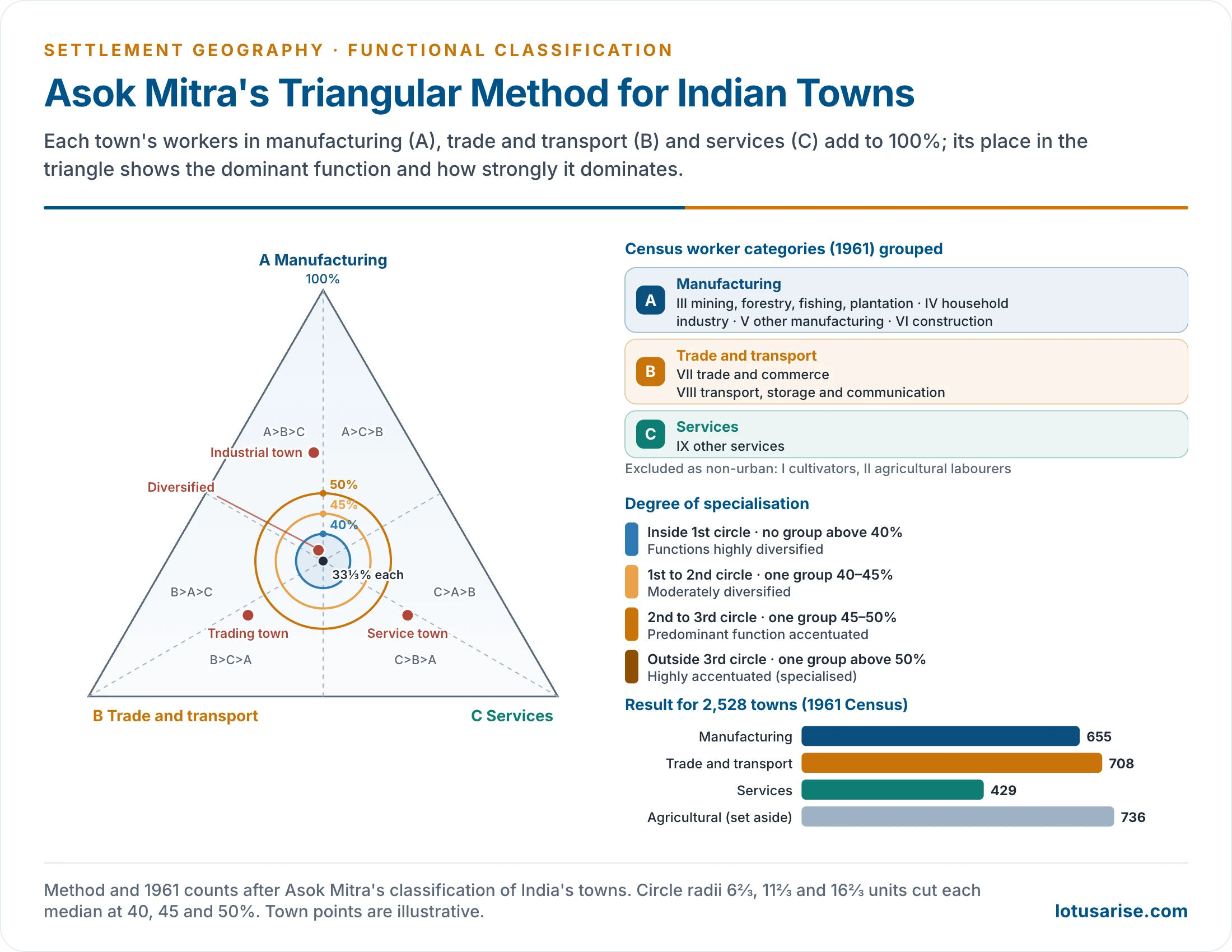
- Results (1961): of 2,528 towns, 736 were agricultural. Of the 1,792 non-agricultural towns, 655 were manufacturing, 708 trade and transport and 429 service towns.
- Of non-agricultural towns that is 36.6%, 39.5% and 23.9%.
- Most towns still show a diversified base. Kolkata came out as highly balanced on the 1964 method and on the later method for both 1961 and 1971 data.
- Merits: simple, uses data available for every town, shows both the type and the degree of specialisation on one graph, and suits Indian census categories.
- Limits: the three groups are broad (mining and construction sit with manufacturing), agricultural towns are set aside rather than classified, and the 40/45/50% circles are conventions.
The Factor-Cluster Classification (1961–1971)
- Asok Mitra and colleagues later classed India’s urban areas by factor analysis and cluster analysis of the worker categories for both 1961 and 1971.
- The clusters did not match neatly between the two censuses, and the final types were not markedly better than those of the triangle. The simple 1964 method remained the practical tool.
- Cluster 8, for example, meant very high transport in 1961 but high trade in 1971.
M. K. Jain’s Classification (1991 Census)
- M. K. Jain, Deputy Registrar General, classified India’s urban agglomerations and towns on 1991 Census data, following Mitra’s logic. It was published by the Office of the Registrar General as an Occasional Paper (No. 3 of 1994).
- Five sectors were formed from the nine industrial categories:
| Sector | Census categories |
|---|---|
| Primary activity | I cultivators, II agricultural labourers, III livestock, forestry, fishing, plantations, IV mining and quarrying |
| Industry | V manufacturing (household and other), VI construction |
| Trade | VII trade and commerce |
| Transport | VIII transport, storage and communication |
| Services | IX other services |
- Unlike Mitra, Jain kept primary activities in, recognising the semi-rural character of many Indian towns.
- Decision rules:
- Mono-functional: one sector employs 40% or more of main workers.
- Bi-functional: no sector reaches 40%, but the two largest together reach 60% or more.
- Multi-functional: no two sectors reach 60%; the three largest are combined.
- Sub-functional categories were added where at least one-quarter of workers were in forestry and fishing, mining, household manufacturing or construction, provided that activity was the first or second function.
- Million-plus cities, 1991:
| Functional category | Cities |
|---|---|
| Industry (IND) | Mumbai, Bengaluru, Ahmedabad, Pune, Surat, Ludhiana, Coimbatore, Varanasi |
| Industry-cum-services | Chennai, Hyderabad, Nagpur, Jaipur, Vadodara, Indore |
| Industry-cum-trade and commerce | Kolkata, Madurai |
| Industry-cum-services-cum-trade and commerce | Kochi |
| Services-cum-industry | Delhi, Kanpur, Visakhapatnam, Bhopal |
| Services | Lucknow, Patna |
- Industry was the first or second function of almost every million-plus city in 1991. Only Lucknow and Patna were purely service cities, and Delhi’s administrative role appeared as services-cum-industry.
- 1991 populations: Mumbai 12,596,243; Kolkata 11,021,918; Delhi 8,419,084; Chennai 5,421,985; Hyderabad 4,344,437; Bengaluru 4,130,288; Ahmedabad 3,312,216; Pune 2,493,987; Kanpur 2,029,889; Lucknow 1,669,204; Nagpur 1,664,006; Surat 1,518,950; Jaipur 1,518,235; Kochi 1,140,605; Patna 1,099,647; Visakhapatnam 1,057,118.
- Assessment: the rules are simple and objective and keep the primary sector in view. But the 40% and 60% cut-points are not justified statistically, the choice of four sub-functions is arbitrary, and labels such as “bi-functional” say little about the degree of specialisation that Mitra’s triangle shows.
Census 2011 and Later Work
- The Census 2011 Primary Census Abstract records workers in four categories: cultivators, agricultural labourers, household industry workers and other workers. Over most of urban India “other workers” dominate, so the four categories alone cannot separate trade, transport, industry and services.
- Its B-series tables (for example B-4) classify main workers by industrial category, based on the National Industrial Classification (NIC). These are the basis of functional classification on 2011 data.
- Town-level tables on industrial categories came out only years after the census. Recent studies use them to class Class I cities by occupational specialisation and to compare the result with Mitra’s 1961 types.
- Long-run shifts visible in such work:
- The service sector has grown in most large cities; many old textile and engineering cities (Mumbai, Kanpur, Ahmedabad) have moved from industry towards trade, finance and services.
- New specialisations have appeared: IT and business services (Bengaluru, Hyderabad, Pune, Gurugram), logistics and warehousing (Bhiwandi), coaching and education (Kota).
- Census towns created in 2011 are often semi-rural, with a sizeable share of primary workers.
- The next census, delayed from 2021, has its population enumeration on a reference date of 1 March 2027. No town-level worker data from it are yet available, so 2011 remains the latest basis.
Evaluation
- Strengths:
- Functional classification goes to the economic base of towns and so explains more than size or form.
- Statistical methods (Nelson, Mitra) made it objective and repeatable, and allowed multiple functions and degrees of specialisation.
- Census-based Indian methods cover every town, giving a national picture that can be repeated at each census.
- Weaknesses:
- Employment is only one measure. It misses the value of output, the reach of a town’s services, its institutions and its hinterland role.
- Thresholds remain conventions, whether Harris’s percentages, Nelson’s +1 SD or Mitra’s 40/45/50% circles.
- Census categories are coarse. “Other services” lumps together administration, education, health, IT and domestic work; informal work is poorly captured.
- Snapshots age fast. Indian cities have changed function rapidly since liberalisation, while town-level census data appear only once a decade and often years late.
- Results depend on the unit used: a municipal town, an urban agglomeration or a metropolitan region can give different answers for the same city.
- Current view: functional classification is best read together with size, hierarchy and morphology. Newer approaches add commuting flows, firm networks and night-light or land-use data to employment, and global schemes rank cities by their connections rather than their workforce alone.
Previous Year Questions
1986Write short note on Functional and hierarchical patterns of Indian cities.1987Write short note on Functional and Morphological Typology of Indian Cities.1990Write short note: Function, classification and hierarchy of urban settlements.2015Discuss Nelson’s method of functional classification of towns.2015“Mono-functional towns are economically vulnerable.” Discuss.2017Mention various methods of functional classification of towns in India and explain the method applied by Asok Mitra.2021Discuss Ashok Mitra’s classification method of Indian cities.





nice note
Good material for UPSC CSE but please add prospective questions with each topic. Thank you!
High, thanks for such concise notes they are simply gold mines.
However one correction, according to Grifith Taylors book “Urban Geography” Chauncey Harris had classified urban cities based on commercial interest. classes were based on employment where he surveyed 984 cities. From there the classification was in 5 categories
Thank you for the systematic notes
Thank u so much for your dedication.loved it.
thank u so much…..
thanks once again