Weber Model of Industrial Location

• Weber’s model of industrial location asks where a factory should stand so that its total cost is lowest. It is the founding statement of least-cost location theory.
• It was set out by Alfred Weber (1868–1958), a German economist and sociologist and the younger brother of Max Weber, in Über den Standort der Industrien (1909). Carl Joachim Friedrich’s English translation, Theory of the Location of Industries, followed in 1929.
• Its core claim: transport cost fixes the first location. Cheap labour and agglomeration can then pull a plant away, but only if the saving beats the extra freight.
• Location theory divides on one question. Weber fixed revenue and varied cost; August Lösch (1940) fixed cost and varied revenue, looking for the site of maximum profit. Other theorists are compared in classical and contemporary location theories.

The Model

Background and Objectives

• The problem had urgency in the late nineteenth century, when railways, coal and urban growth were redrawing the industrial map. Wilhelm Launhardt (1882) had already posed the three-point problem. Weber turned it into a general theory, with a mathematical appendix by Georg Pick.
• It is a normative, deductive model: it says where a rational firm should locate under stated conditions, and it serves as a yardstick for measuring departures from that ideal. Weber called this his “pure” theory.
• Objectives:
  • to find the minimum-cost location of an industry;
  • to show that transport cost is the most fundamental location factor;
  • to frame labour and agglomeration as deviations from the transport-cost optimum.

Assumptions

Group	Assumption
Space	Isotropic surface: uniform in physiography, climate and culture
Economy	A self-contained region under perfect competition, with stable politics
Actors	Rational economic men who minimise cost
Raw materials	Deposits and ubiquities at known, fixed places
Market	Consumption at given points; demand and price fixed, so least cost means highest profit
Transport	One mode, equal connectivity; freight rises in proportion to weight and distance
Labour	Immobile, at fixed places, each with its own wage and unlimited supply

• The labour assumption is often misquoted. Wages must differ between places, or there would be no labour deviation to analyse.
• Bulk or difficulty of handling can be converted into an equivalent extra weight, which Weber called ideal weight. Freight rates can therefore be treated as uniform.

Factors of Location

• Weber sorted location factors twice over:
  • general factors affect every industry; special factors affect only some, such as perishability or humidity;
  • regional factors distribute industry between places; agglomerative and deglomerative factors then concentrate or scatter it within that pattern.
• He found two general regional factors, transport and labour, and one general agglomerative factor. Hence the three-step argument: find the transport optimum, adjust for labour, adjust for agglomeration.

Key Terms

Term	Precise meaning
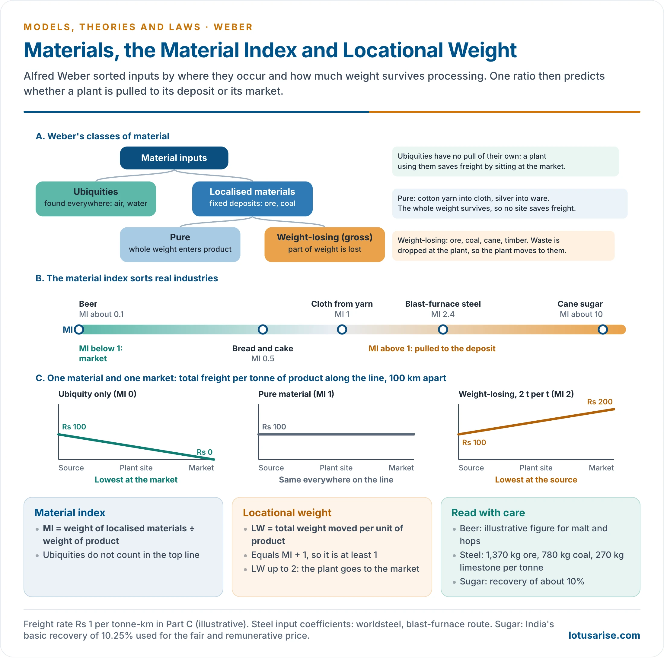
Ubiquities	Materials available everywhere at the same price, such as air and, in the model, water. They exert no pull of their own
Localised materials	Materials found only at fixed deposits, such as ores and coal
Pure material	A localised material whose whole weight enters the product, such as yarn woven into cloth
Weight-losing (gross) material	A localised material only part of whose weight enters the product, such as ore, cane and timber; coal is the extreme case, leaving no weight in the product
Material index (MI)	Weight of localised materials ÷ weight of the product
Locational weight (LW)	Total weight moved per unit of product: localised materials plus the product itself. So LW = MI + 1
Locational figure	The triangle or polygon joining deposits and market
Isotim	Line through points of equal transport cost for one item, a single material or the product
Isodapane	Line through points of equal total transport cost, all materials and the product together. Weber drew it as equal additional cost above the least-cost point
Critical isodapane	The isodapane whose additional freight exactly equals the saving offered at a labour or agglomeration site
Labour index	Average labour cost per tonne of product
Labour coefficient	Labour index ÷ locational weight; it measures how far labour can pull a plant
Coefficient of manufacture	Value added per tonne of locational weight; it measures the tendency to agglomerate

• Isophane sometimes appears in older writing as a slip for isodapane; it has no separate meaning in location theory. The word isotim came later, from Tord Palander (1935).

The Material Index Rule

• The MI predicts orientation in a single number:
  • MI below 1: ubiquities add weight, so the product is heavier than what is hauled to the plant. The pull is to the market. Beer, soft drinks and bakery goods are examples.
  • MI of 1: only pure materials. With one material the plant may stand anywhere on the line between source and market, since total freight does not change. With two or more, it goes to the market.
  • MI above 1: weight is lost in processing, and the pull is to the deposit if one material dominates.
• Weber’s own rule: any industry with MI not above 1, and so LW not above 2, lies at the place of consumption. Only weight-losing materials can draw a plant to a deposit.
• Real values:

Product	Inputs	MI	Pull
Beer	Malt and hops; most of the weight is water (illustrative)	About 0.1	Market
Bread, cake	Sugar 1 t + flour 1 t + water and other ubiquities, making 4 t	0.5	Market
Cloth from yarn	Yarn 10 t makes 10 t	1	Footloose along the line
Steel, blast-furnace route	1,370 kg ore, 780 kg coal, 270 kg limestone per tonne (worldsteel)	About 2.4	Materials
Cane sugar	Recovery of about 10% in India	About 10	Cane belt

Transport Orientation

One Material, One Market

• Weber’s simplest figure is a line (linear location) between a source and a market, with three outcomes:
  • Ubiquitous material: the plant goes to the market, because moving the product is the only freight.
  • Pure localised material: total freight is the same anywhere on the line. Terminal handling tips the choice to one end in practice.
  • Weight-losing material: the plant goes to the source, so that the waste is never hauled.

Two Materials, One Market: The Locational Triangle

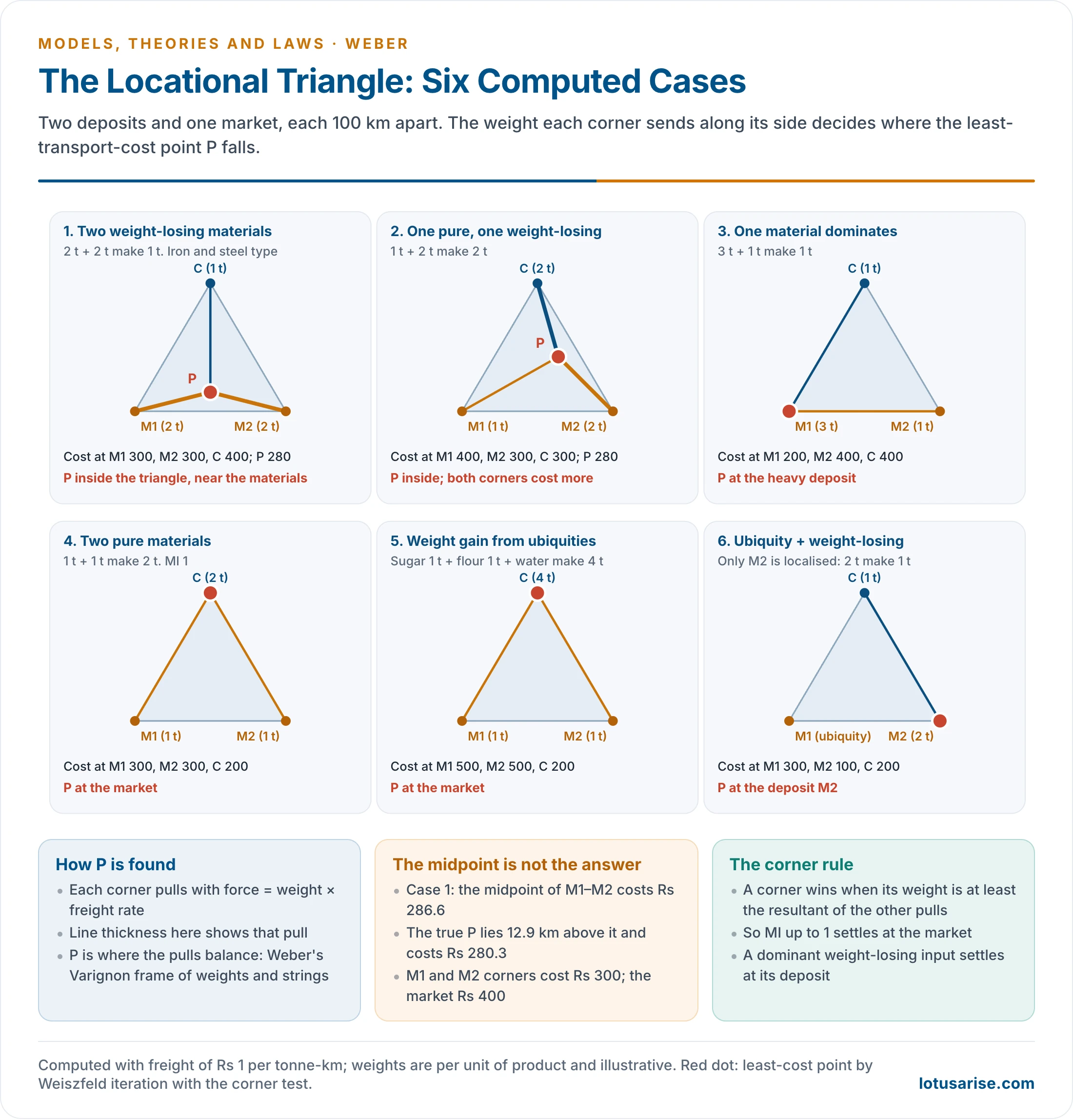
• Two deposits (M1 and M2) and one market (C) form the locational triangle, also called the weight triangle when its corners are read as pulls. More materials or markets give a locational polygon.
• Transport cost at any site is weight × distance, summed over the three corners. Each corner therefore pulls with a force equal to its weight. The balancing point P is the least-transport-cost location.
  • Weber’s appendix solves it mathematically. A Varignon frame of strings and weights solves it physically.
• A worked example. Corners are 100 km apart and freight is Rs 1 per tonne-km. Two materials of 2 t each make 1 t of product.

Site	Calculation	Total freight
At M1 or M2	(2 × 100) + (1 × 100)	Rs 300
At the market C	(2 × 100) + (2 × 100)	Rs 400
Midpoint of M1 and M2	(2 × 50) + (2 × 50) + (1 × 86.6)	Rs 286.6
P, the true optimum	12.9 km above that midpoint	Rs 280.3

• The midpoint is not the answer, because the product also pulls. P lies towards the market by exactly as much as the weights require.

The Possible Cases

Materials	Example	Outcome
Both ubiquitous	Water and air only	At the market
One ubiquitous, one weight-losing	2 t makes 1 t with free water	At the deposit
One pure, one weight-losing	1 t + 2 t makes 2 t	Inside the triangle; better than either corner
Both pure	1 t + 1 t makes 2 t	At the market, since MI is 1
Both pure, with ubiquities added	Sugar, flour and water make cake	At the market, firmly
Both weight-losing, balanced	Ore and coal to steel	Inside, nearer the materials
One weight-losing, dominant	3 t + 1 t makes 1 t	At the heavy deposit

• The corner rule: a corner wins when its weight is at least equal to the resultant pull of the other two. A material weighing as much as all the rest combined always wins.

Isotims and Isodapanes

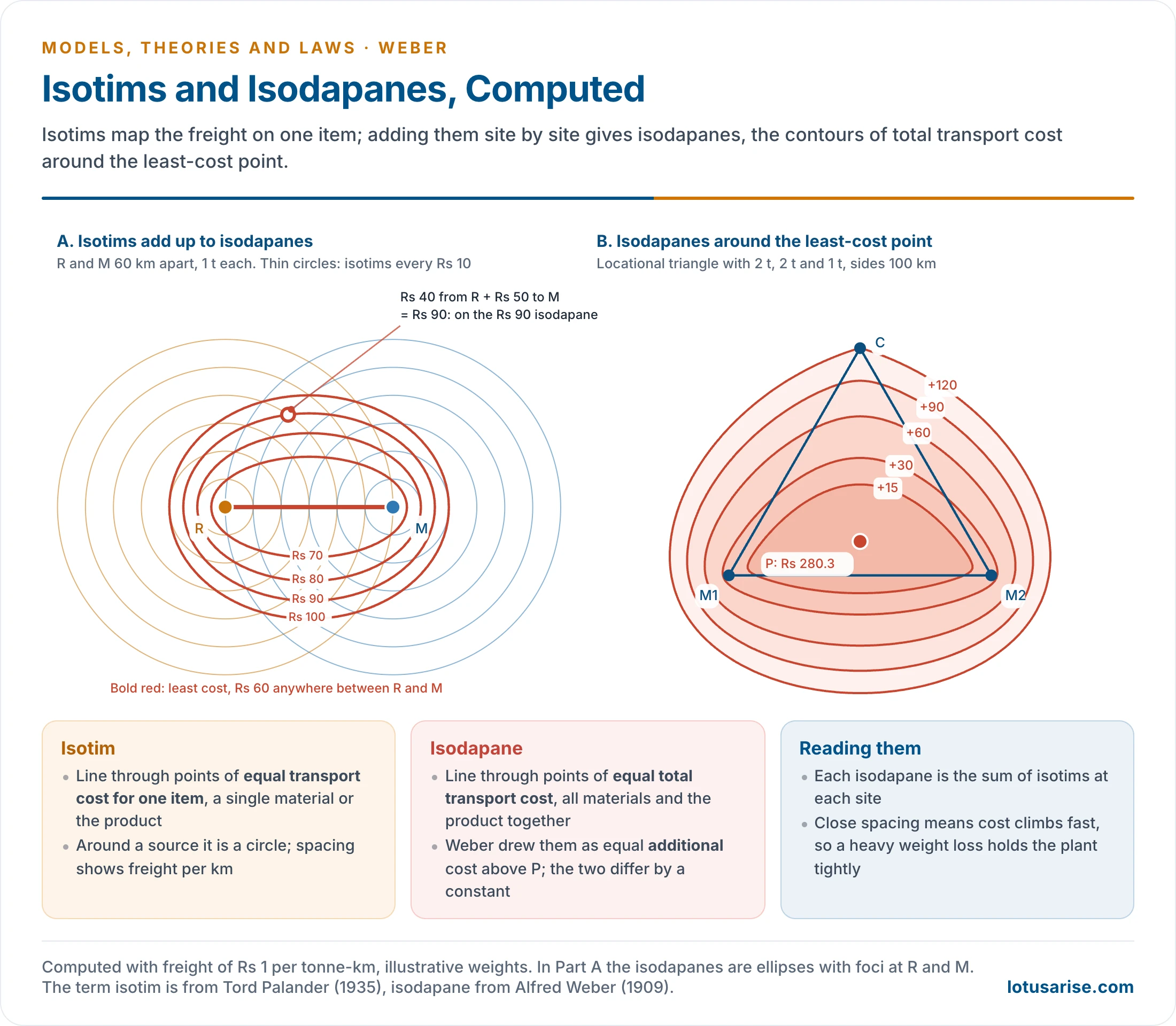
• Isotims map one item’s freight. Around a source they are concentric circles, spaced by freight per km, so a heavier item has closer circles.
• Isodapanes come from adding isotims site by site. If a site is Rs 40 from the material and Rs 50 from the market, it lies on the Rs 90 isodapane.
  • With equal weights on a line they are ellipses, with the two points as foci and a straight line of least cost between them.
  • With a locational triangle they are ovals around P.
• Their spacing carries the message. Tightly packed isodapanes mean that cost climbs fast with distance from P, so the plant is held firmly. Wide spacing means that it can move cheaply.

The Two Deviations

Labour Deviation

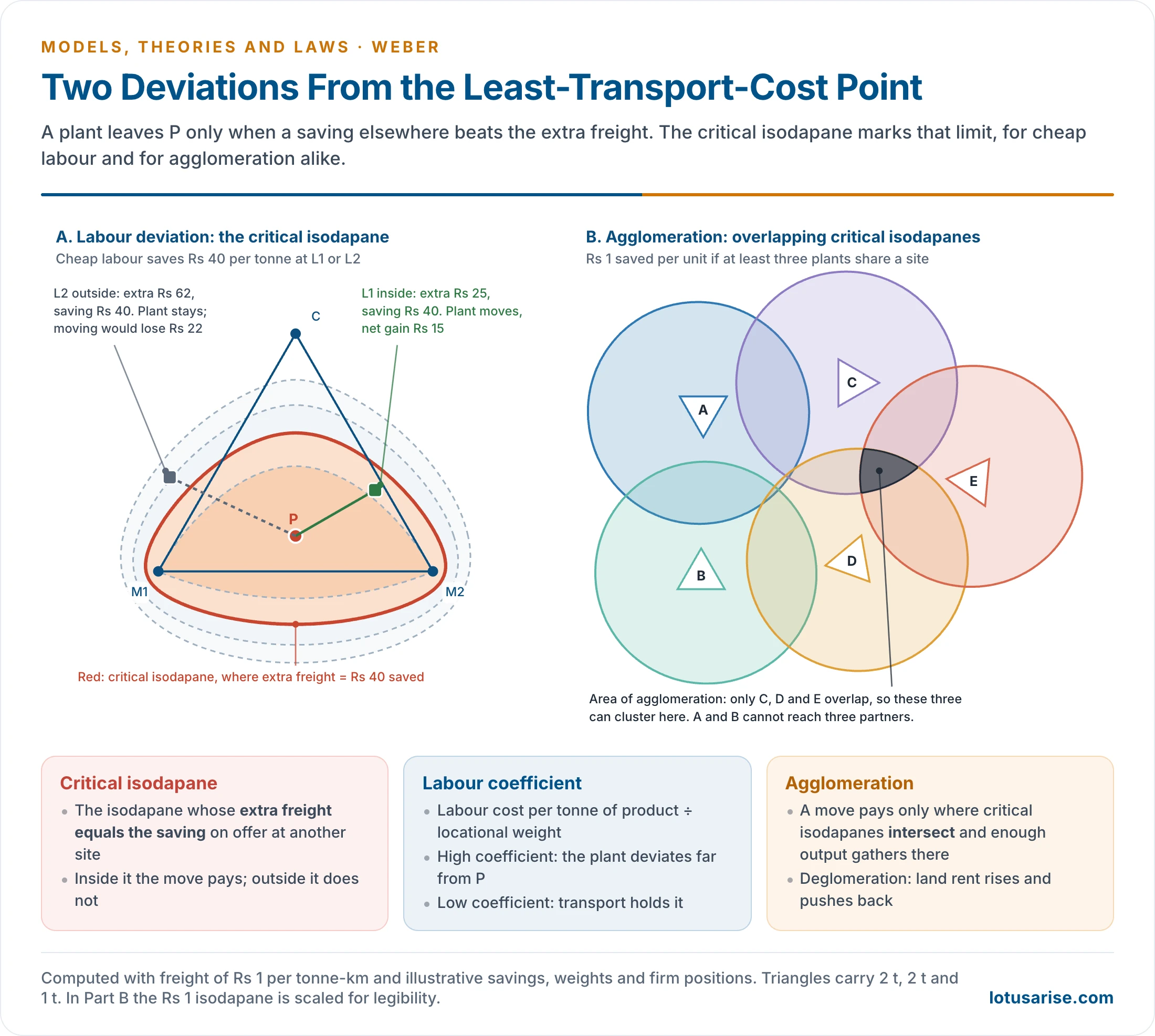
• A plant moves from P to a cheap-labour site only if the saving per tonne exceeds the extra freight per tonne.
• Draw isodapanes around P. The critical isodapane is the one whose value equals the labour saving.
  • A labour site inside it attracts the plant, because the saving is greater than the added freight.
  • A labour site outside it does not.
• Worked example: a site saves Rs 40 per tonne in wages. At site L1, on the +Rs 25 isodapane, the plant moves and gains Rs 15. At site L2, on the +Rs 62 isodapane, moving would lose Rs 22, so the plant stays at P.
• The same test in total costs, with illustrative figures for a plant whose labour bill is Rs 500 per tonne at P:

Site	Freight	Labour	Total per tonne	Verdict
Least-transport-cost point P	Rs 400	Rs 500	Rs 900	Benchmark
Cheap-labour site, 120 extra	Rs 520	Rs 250	Rs 770	Moves: Rs 250 saved for Rs 120 extra
Cheap-labour site, 300 extra	Rs 700	Rs 250	Rs 950	Stays: the saving is smaller than the extra freight

• Two measures decide how strong the pull is:
  • a high labour coefficient lets an industry deviate far. Garments and footwear have much labour and little weight, and have moved from one low-wage country to the next: Bangladesh and Vietnam, for example, or Tiruppur within India.
  • a low coefficient ties a plant to P. Steel and cement carry too much weight to chase wages.
• Environmental conditions matter too. Dense populations create labour pools, and better transport lowers freight per km, spreading the isodapanes. Falling freight therefore strengthens labour orientation over time, a result Weber drew himself.

Agglomeration Deviation

• Agglomeration is a saving that arises when production gathers at one place. Weber distinguished two stages:
  • enlargement of the plant, or scale economies;
  • association of plants, sharing specialised equipment, organised labour, bulk purchase and marketing, and general overheads such as gas, water and roads.
• Deglomeration is the opposing force, chiefly the rise in land rent where firms crowd together.
• The geometry repeats the labour case. Each plant has a critical isodapane set by the saving on offer. Plants can gain only where those isodapanes overlap, and the overlap must hold enough output to earn the saving.
  • In the standard illustration, a saving of Re 1 a unit needs at least three plants on one site. If only firms C, D and E share an overlap, those three can cluster, and firms A and B stay put.
• Industries with a high coefficient of manufacture, which add much value per tonne, agglomerate most readily.
• Indian and world examples: the Chakan–Pune automobile belt, Tiruppur knitwear, Bengaluru software, and policy forms such as Special Economic Zones and industrial corridors.
• New Economic Geography later made this deviation its central subject. Weber had treated it as a local adjustment.

Applications

United States: A Weight-Losing Test

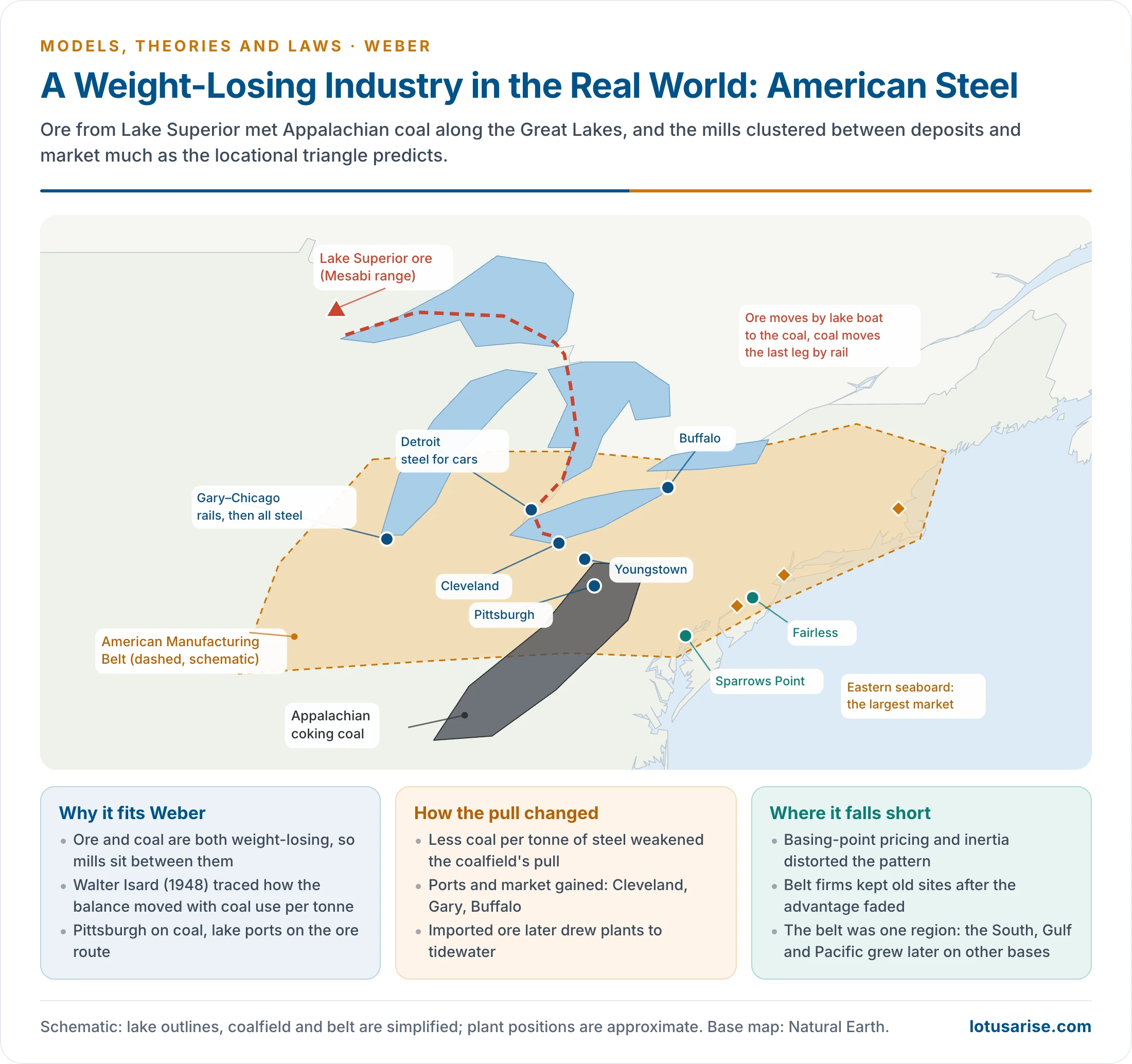
• Walter Isard (1948) traced the location of American iron and steel against Weber’s logic. Ore came from Lake Superior, coking coal from the Appalachians, and the market lay along the eastern seaboard and in the Midwest.
• Mills gathered between the deposits and the market: Pittsburgh and Youngstown near the coal, and Cleveland, Buffalo and Gary–Chicago on the lake route. Detroit grew on the car industry’s demand.
• As technical progress cut coal use per tonne, the pull of the coalfield weakened and lake ports and markets gained. Imported ore later drew plants such as Sparrows Point and Fairless to tidewater.
• Wilfred Smith’s work on weight-losing industries in Britain gave similar support. The wider world pattern of manufacturing regions reflects many other forces as well.

Europe: A Weight-Gaining Case

• Bakery, brewing and soft-drink plants remain spread with population and concentrated near the great urban markets of north-west Europe, because they add water and bulk close to the consumer.

India: Jamshedpur and the Steel Shift

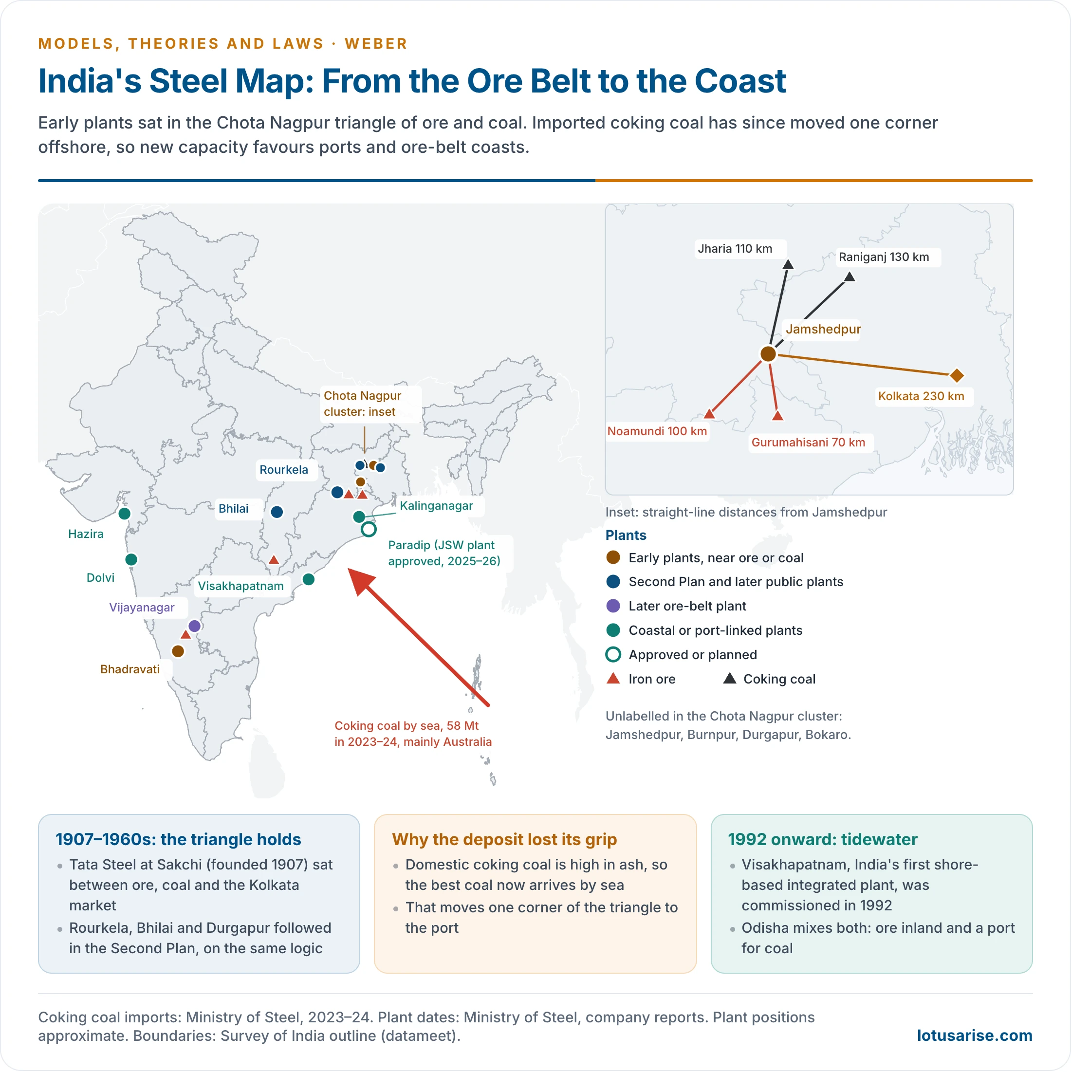
• Tata Steel at Sakchi (Jamshedpur) is the classic triangle. It was founded in 1907 and made its first steel in 1912.
  • Iron ore: Noamundi about 100 km and Gurumahisani about 70 km away, in straight-line distance.
  • Coking coal: Jharia about 110 km and Raniganj about 130 km away.
  • Market and port: Kolkata about 230 km away.
  • Water: the Subarnarekha and Kharkai rivers. Labour: the tribal and rural Chota Nagpur region, Bihar and Odisha.
• Durgapur, Rourkela and Bhilai of the Second Five Year Plan followed the same ore-belt logic, though choice of site was also a state decision.
• Three things have since moved the triangle:
  • Imported coal. Most domestic coking coal is high in ash. India imported 58 Mt in 2023–24, mainly from Australia (Ministry of Steel), so one corner of the triangle now lies at a port.
  • Lower material use and new routes. Efficiency reduces the MI. Over half of India’s crude steel in 2023–24 came from electric arc and induction furnaces, which use scrap and sponge iron and can stand nearer markets.
  • Policy. The freight equalisation scheme for steel and coal, which ran from 1952 until the early 1990s, removed the very advantage Weber’s model rests on, and helped steel users set up far from the ore belt.
• Coastal capacity: Visakhapatnam (commissioned 1992) was India’s first shore-based integrated plant. Hazira and Dolvi serve the western markets, and Odisha combines inland ore with ports. JSW’s board approved a 5 Mt plant at Paradip in 2025–26. Coal arrives by sea, ore comes down by rail, and steel leaves through the same ports.
• The National Steel Policy 2017 targets 300 Mt of capacity by 2030–31, against about 180 Mt in 2023–24.

Other Present-Day Cases

• Aluminium splits along the chain. Bauxite loses most of its weight, so alumina refineries stand near mines, as at Damanjodi in Odisha. Smelting then follows cheap power, as at Angul. Weber treated fuel as a weight-losing material that leaves no weight in the product, and power plays that role here.
• Sugar stays in the cane belt, since cane is weight-losing and spoils quickly after cutting.
• Cement also splits. Limestone loses much of its weight in the kiln, so clinker is made near the quarry, in belts such as Satna and Chandrapur. Grinding units then stand near markets and ports, because the finished product is cheap and bulky. One industry thus follows the deposit at one stage and the market at the next, which Weber’s single point cannot show.
• Electric vehicles. Batteries are heavy, so gigafactories are placed close to car assembly, and assembly in turn follows markets and policy.
• Semiconductors and software. Very little weight and very high value make freight almost irrelevant. Chip plants at Dholera and Sanand rest on subsidy, power, ultra-pure water and skills. Software follows talent. These footloose industries lie outside the transport logic while keeping to the logic of agglomeration.

Evaluation

Criticism

• Unreal assumptions: isotropic surfaces, perfect competition and rational actors with full knowledge do not exist. Real firms choose from a range of acceptable sites.
• Demand ignored: the theory takes demand and price as fixed, though prices move with supply and demand. Lösch (1940) made demand the central variable, and his maximum-revenue approach is the sharpest rival.
• Transport oversimplified:
  • freight is not proportional to distance, because rates taper with long hauls and carry terminal charges, as Edgar M. Hoover (1937, 1948) showed;
  • raw materials often travel at lower rates than finished goods;
  • break-of-bulk points and ports become natural sites, a case missing from the triangle.
• Too much weight on transport: labour and agglomeration are measured only through it. In modern industry, processing cost, technology and skills often matter more.
• Fixed points: real firms use many materials, sell in many markets and buy from alternative sources. Cotton textiles in India, for example, sell nationwide.
• Labour treated too simply: wages and productivity both vary, labour migrates, and skill matters as much as price.
• Fixed coefficients: Weber allowed no substitution between inputs. Walter Isard (1956) and Leon Moses (1958) showed that firms trade freight against other inputs.
• Agglomeration under-analysed: space problems, congestion and energy limits get little attention, and the theory says little on who moves first.
• History and inertia left out: Mumbai, Kolkata and Delhi kept their lead after 1947 because of what was already there.
• Politics and institutions left out: tariffs, licensing, public-sector plants and backward-area incentives can reverse the expected pattern. An exporter will often prefer a port to the least-cost point.
• Dated firm: the single-plant, single-product firm has given way to multi-plant transnational corporations and value chains.
• Behaviour: entrepreneurs act on partial knowledge and settle for sub-optimal sites, the argument of the behavioural matrix.

Strengths

• It was the first general theory of industrial location, and it replaced lists of location factors with a single method: measure each pull in the same unit, money per tonne of product.
• It gave later writers their tools. Isotims, isodapanes and spatial substitution run through Palander, Hoover, Isard and David M. Smith.
• It predicts the weight-losing case well, as tests on steel in the United States and Britain showed, and it still reads correctly for sugar, cement and smelting.
• It separates general causes from accidents of place, which is why it remains a teaching model and a planning benchmark.

What Survives

Principle	Status today	Illustration
Transport	Weaker overall, but valid for bulk and weight-losing goods; the relation between weight, distance and cost still holds	Cement, sugar, steel at ports
Labour	Skill often matters more than wage, yet low wages still attract labour-intensive stages	Garments in Bangladesh and Vietnam
Agglomeration	The strongest survivor	Clusters, SEZs, export zones, Silicon Valley

• Falling freight has shifted the weight from the first of Weber’s three factors to the third. Refrigerated transport now takes even Gujarat’s milk products to distant metros.
• Weber himself accepted that “pure” rules needed testing against local, social and political conditions. His method of finding the least-cost point and then measuring each deviation is still the logic of site selection, now run on GIS and location models.

Aspect	Alfred Weber (1909)	August Lösch (1940)
Goal	Least cost	Maximum profit
Fixed	Demand and price	Production cost
Varies	Transport, labour, agglomeration	Demand and market area
Spatial form	Triangle and isodapanes	Hexagonal market areas
Main limit	Ignores demand	Treats cost as uniform

Summary

Category	Details
Author	Alfred Weber (1868–1958), German economist
Work	Über den Standort der Industrien, 1909; English 1929
Core idea	Least-cost location: transport first, then labour and agglomeration
Key tools	Material index, locational weight, locational triangle, isotim, isodapane, critical isodapane
Rule	MI up to 1: market. High MI with a dominant material: deposit
Tests	Isard on US steel; Jamshedpur and the Indian steel belt
Main critique	Ignores demand, rigid transport and labour, no behaviour or institutions
Value today	Yardstick for site selection; agglomeration remains central