- Thermohaline circulation is the slow, density-driven movement of ocean water. The name joins thermo (heat) and haline (salt), the two properties that set the density of seawater.
- Winds drive the surface currents of roughly the upper tenth of the ocean. Density differences created at the surface move the other 90%, the deep and bottom waters below the pycnocline.
- The Atlantic Meridional Overturning Circulation (AMOC) is its Atlantic branch: warm water flows north near the surface, sinks in the subpolar North Atlantic and returns south at depth. It carries heat that keeps north-western Europe mild, and its possible collapse is one of the most debated climate tipping points.
Thermohaline Circulation

How density drives the deep ocean
- Density rises with cooling, evaporation and sea-ice formation, which leaves salt behind in the water (brine rejection). Density falls with heating, rain, river runoff and melting ice.
- All these processes act at the surface. Once a parcel of water sinks, its temperature and salinity change only by slow mixing, so it keeps its identity as a water mass for centuries.
- Thermohaline convection: cold or salty surface water becomes denser than the water below, sinks, and is replaced by lighter water drawn in at the surface.
- Sinking to great depth happens in very few places.
- In the tropics a strong thermocline and pycnocline cap the warm surface layer. Water pushed down at convergences spreads out just below it.
- In the middle latitudes winter convection stirs only a thin layer.
- Deep and bottom water form only at high latitudes, where salty water is cooled (the North Atlantic) or brine is rejected under sea ice (the Antarctic shelves).
- Upwelling is spread out. Deep water returns slowly through the whole ocean interior, and fastest around Antarctica, where divergence of the surface water lifts it up.
- Deep flows are slow, a few kilometres to a few tens of kilometres a year, except in narrow deep western boundary currents. Henry Stommel and Arnold Arons (1960) showed how the Earth’s rotation concentrates them along the western sides of the basins.
Temperature, salinity and density as causes of circulation
- Temperature: the warm, light water of low latitudes stands slightly higher than cold polar water. It flows poleward at the surface, and cold water returns equatorward at depth to complete the loop.
- Salinity: where evaporation exceeds precipitation (the subtropics, enclosed seas) water turns salty and dense. Lighter, fresher water flows in at the surface to replace what sinks.
- Fresh water from rain, rivers and ice melt lowers density and raises sea level locally. The East Greenland Current is partly a melt-water outflow.
- Density combines all three, together with pressure. Its horizontal differences set up pressure gradients, which the Coriolis force turns into geostrophic deep currents.
- Marginal seas show the mechanism in miniature. A two-layer exchange forms at each strait:
| Strait | Surface flow | Deep flow | Cause |
|---|---|---|---|
| Gibraltar | Atlantic water into the Mediterranean | Salty Mediterranean water out to the Atlantic | Evaporation exceeds rain and runoff |
| Bab-el-Mandeb | Gulf of Aden water into the Red Sea | Very salty Red Sea water out | Intense evaporation; outflow strongest in winter |
| Danish straits | Brackish Baltic water out to the North Sea | Salty North Sea water in | Large river inflow freshens the Baltic |
- The older debate. By about 1870 oceanographers argued over whether wind stress or density differences between equatorial and polar water drove the currents.
- Vilhelm Bjerknes’s circulation theorem (1898) made it possible to calculate density-driven currents from measured temperature and salinity, the dynamic method.
- Vagn Walfrid Ekman (1905) explained wind-driven flow. Today the two are seen as working together: winds dominate the surface, density the deep ocean.
| Feature | Wind-driven circulation | Thermohaline circulation |
|---|---|---|
| Driver | Wind stress, with Coriolis force | Density differences from heat and freshwater fluxes |
| Depth | Upper few hundred metres | Intermediate, deep and bottom waters |
| Share of ocean volume | About 10% | About 90% |
| Speed | Up to 1–2 m/s in boundary currents | Centimetres per second or less |
| Pattern | Gyres, equatorial currents, upwelling | Sinking at high latitudes, slow spreading, diffuse upwelling |
| Time to renew | Years to decades | Centuries to about a thousand years |
The modern view: winds and tides power the “density-driven” flow
- Johan Wilhelm Sandström (1908) showed that heating and cooling at the same level, the sea surface, cannot by themselves keep a strong circulation going.
- Walter Munk and Carl Wunsch (1998) estimated that about 2 terawatts of mixing energy from tides and winds are needed to lift dense deep water back through the stratified interior.
- Westerly winds over the Southern Ocean pull deep water up to the surface along sloping density surfaces. This wind-driven upwelling closes much of the loop.
- Many oceanographers therefore prefer the term meridional overturning circulation. Density sets where water sinks; wind and tidal mixing supply much of the energy that brings it back up.
Deep-water formation
- North Atlantic Deep Water (NADW) forms in winter in the Labrador, Irminger and Nordic (Greenland–Norwegian) Seas.
- The Gulf Stream and North Atlantic Current carry salty subtropical water north. Winter cold strips its heat until it sinks to 1,500–4,000 m.
- Dense water from the Nordic Seas spills south over the Greenland–Scotland Ridge, through the Denmark Strait and the Faroe Bank Channel.
- The OSNAP array (data from 2014) showed that most of the overturning happens east of Greenland, in the Irminger and Iceland basins, rather than in the Labrador Sea as models had suggested.
- Antarctic Bottom Water (AABW), the densest water in the open ocean, forms on the Antarctic shelves of the Weddell Sea, the Ross Sea, the Adélie Land coast and Cape Darnley.
- Sea ice forming in coastal polynyas rejects brine. The cold, salty shelf water cascades down the slope and mixes with Circumpolar Deep Water.
- Why the Pacific, Arctic and Indian Oceans form no deep water:
- The North Pacific surface is too fresh (salinity about 32–33).
- The Arctic is capped by fresh water from the Siberian rivers, and its deep basins are walled off by ridges. The Bering Strait is about 85 km wide and only about 50 m deep, and the Fram Strait is the only deep gateway to the Atlantic.
- The Indian Ocean is closed by land at about 25°N, so it has no northern polar source.
- Bottom relief steers the deep flow. Ridges and sills decide where dense water can pass, and narrow gaps such as the Vema Channel in the South Atlantic funnel AABW northward. The individual water masses are traced by their temperature, salinity and oxygen.
The global conveyor belt
- Wallace Smith Broecker introduced the “great ocean conveyor” image in 1987 to show the overturning as one connected loop through all the oceans.
- The path:
- NADW flows south through the western Atlantic and joins the Antarctic Circumpolar Current, mixing with AABW and deep water from round Antarctica.
- This mixed deep water spreads north into the Indian and Pacific Oceans, where it slowly rises and warms.
- Surface water returns to the Atlantic by a warm route, through the Indonesian Throughflow and round the Cape of Good Hope as Agulhas leakage, and a cold route through the Drake Passage.
- In the Atlantic it is carried north by the Gulf Stream to the sinking regions, and the loop starts again.
- A full circuit takes around a thousand years. The deep North Pacific holds the oldest water in the ocean, the poorest in oxygen and richest in nutrients.
- What the conveyor does:
- Heat: it moves heat poleward, especially in the Atlantic.
- Ventilation: it carries oxygen into the deep ocean.
- Nutrients: organic matter keeps sinking into the deep water as it ages, so upwelling regions are fertile.
- Carbon: sinking water stores carbon in the deep ocean for centuries. This makes the North Atlantic and the Southern Ocean major carbon sinks.
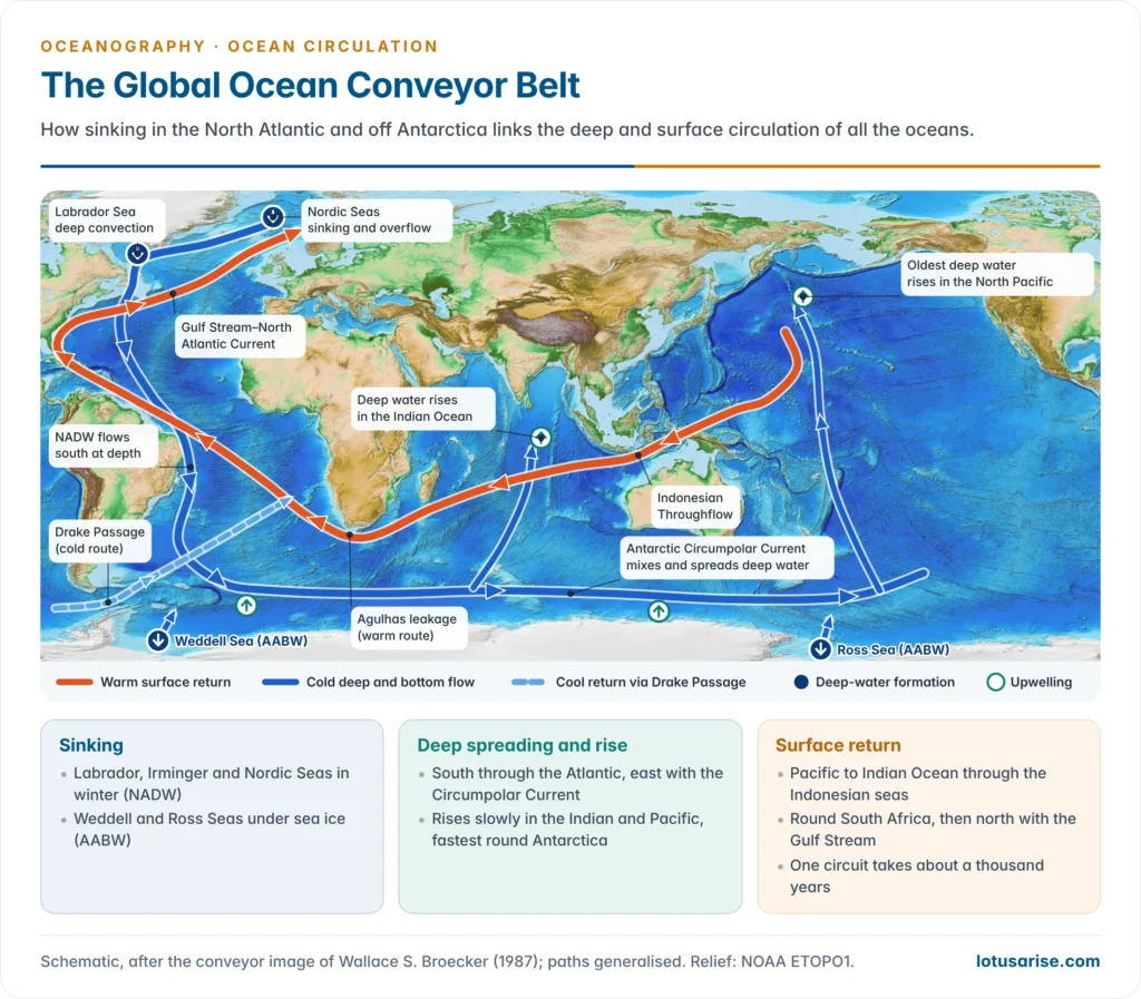
- The metaphor is simplified. Floats and tracers show that deep water spreads through eddies and many interior pathways, not one steady ribbon, as M. Susan Lozier (2010) stressed. The image remains a sound first summary of how the overturning links the oceans.
The Atlantic Meridional Overturning Circulation
Structure and strength
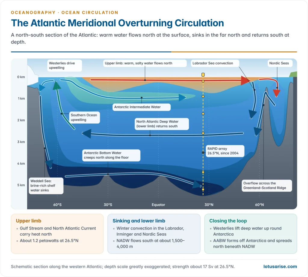
- The upper limb is warm, salty water carried north by the Gulf Stream and the North Atlantic Current.
- The lower limb is cold NADW returning south at about 1,000–4,000 m, mainly in the Deep Western Boundary Current. Beneath it, a weaker abyssal cell of AABW creeps north along the floor.
- Strength is measured in sverdrups (1 Sv = 1 million m³ per second). The AMOC averages about 17 Sv at 26.5°N, roughly 80 times the discharge of the Amazon.
- Heat: it carries about 1.2 petawatts northward at 26.5°N. The Atlantic is the only ocean that moves heat northward at every latitude, even south of the equator, so its overturning dominates the ocean’s heat budget in the north.
- The Gulf Stream is not the AMOC. It is mainly wind-driven and will keep flowing as long as the westerlies and trades blow. Only the part of its flow that feeds the overturning would be lost.
- Why it can tip: the salt-advection feedback. Henry Stommel (1961) showed that a circulation of this kind can have two stable states.
- The AMOC brings salt north, which keeps the sinking regions dense and the circulation running.
- If enough fresh water is added, sinking weakens, less salt arrives, and the water freshens further. Past a threshold the circulation can switch to a weak or collapsed state and stay there.
Monitoring the AMOC
- The RAPID array at 26.5°N has measured the AMOC continuously since April 2004. It is run jointly by British and US institutions.
- Moorings record density profiles at the western and eastern boundaries and on the Mid-Atlantic Ridge, from which the deep flow is calculated geostrophically.
- A submarine cable across the Straits of Florida measures the Florida Current, and satellite winds give the shallow Ekman transport.
- Other arrays now cover the basin: MOVE at 16°N, SAMBA at 34.5°S and OSNAP in the subpolar North Atlantic (from 2014). All give means of about 16.7–17.3 Sv.
- Indian research works at the southern end of the loop: NCPOR’s Southern Ocean expeditions sample the Antarctic source waters, and the Indian Argo programme of INCOIS tracks the warming and freshening of the Indian Ocean that feeds the warm return route.
- Before 2004, the AMOC is reconstructed from proxies: a sea-surface “cold blob” south of Greenland, sediment grain size from deep currents, and repeated ship sections.
Observed changes
- RAPID record: strength fell from about 18–19 Sv (2004–08) to about 15–17 Sv (2011–20), with a sharp 30% dip in 2009–10. Much of the 2007–11 drop is put down to natural changes in wind and buoyancy forcing.
- An analysis of 2004–2023 data (2025) found a weakening of about 1 Sv per decade (range 0.4–1.6). This matches climate-model projections and does not point to a mid-century collapse.
- Longer reconstructions disagree:
- Levke Caesar and Stefan Rahmstorf (2018), using the cold-blob fingerprint, estimated a decline of about 15% (about 3 Sv) since the mid-20th century. A 2021 proxy synthesis found the AMOC weaker than at any time in the last thousand years.
- Jens Terhaar and colleagues (2025), using air–sea heat fluxes, found no decline in decadal-mean strength from 1963 to 2017.
- IPCC AR6 (2021) has only low confidence in any 20th-century trend. The direct record is still too short to separate a human signal from natural variability.
Projections and the tipping-point debate
- IPCC AR6:
- The AMOC will very likely weaken over the 21st century under all emission scenarios: by about 24% (range 4–46%) under a low-emission pathway and 39% (17–55%) under a very high one.
- It has high confidence in the decline but low confidence in its size.
- It has medium confidence that there will be no abrupt collapse before 2100.
| Line of evidence | Study | Finding |
|---|---|---|
| Statistical early-warning signals | Niklas Boers (2021) | Rising variance and memory in temperature and salinity records suggest loss of stability |
| Statistical forecast | Peter and Susanne Ditlevsen (2023) | Collapse between 2025 and 2095, most likely around 2057 |
| Physics-based indicator | René van Westen, Michael Kliphuis and Henk Dijkstra (2024) | Freshwater transport at the southern edge of the Atlantic shows the AMOC “on tipping course” |
| Extended model runs | Sybren Drijfhout and colleagues (2025) | Deep winter convection collapses by mid-century in many runs; overturning shuts down after 2100 in some low- and medium-emission runs too |
| Observation-constrained models | Bonan and colleagues (2025) | Weakening limited to about 18–43% by 2100; collapse unlikely this century |
| 34 climate models under extreme forcing | Jonathan Baker and colleagues (2025) | AMOC weakens but survives, held up by wind-driven Southern Ocean upwelling |
| Observation-constrained models | Portmann and colleagues (2026) | About 51% weakening by 2100 under a medium-emission pathway |
| Model precursor | van Westen and Dijkstra (2026) | An abrupt northward jump of the Gulf Stream path precedes collapse by decades; a gradual northward shift is already seen |
- Why the experts disagree:
- The records are short. RAPID has about two decades of data, and proxies carry wide errors.
- Models may be too stable. Many get the sign of the Atlantic’s freshwater transport wrong and leave out Greenland meltwater.
- Early-warning statistics assume an idealised system and cannot give a reliable date.
- “Collapse” is defined differently, usually as a fall below about 6 Sv. Even then the switch would unfold over decades to a century.
- Not every influence pushes towards collapse. A 2019 modelling study found that faster Indian Ocean warming can partly strengthen the AMOC: heavier rain over the Indian Ocean reduces rain over the Atlantic, making it saltier and denser.
- The balance of evidence is that the AMOC is weakening and will weaken further. A collapse this century is considered unlikely but cannot be ruled out, and its consequences would be severe enough to treat it as a serious risk.
- In October 2024 more than 40 climate scientists from 15 countries urged the Nordic Council of Ministers to assess the risk seriously.
- In November 2025 Iceland designated a possible collapse a national security concern.
Palaeo-evidence of past AMOC shifts
- Glacial climate was unstable. During the last ice age the AMOC was shallower and weaker and switched repeatedly between strong and weak modes.
- Dansgaard–Oeschger events: abrupt Greenland warmings of several degrees within decades, followed by slow cooling.
- Heinrich events: armadas of icebergs released from the Laurentide ice sheet. Hartmut Heinrich (1988) identified them from layers of ice-rafted debris on the North Atlantic floor. The melt-water slowed or halted the overturning.
- The Younger Dryas (about 12,900–11,700 years ago) returned the North Atlantic region to near-glacial cold during deglaciation.
- The leading explanation is a melt-water pulse, possibly from glacial Lake Agassiz, that freshened the North Atlantic and slowed the AMOC. The trigger and route are still debated.
- The bipolar seesaw: when the AMOC weakened, the North cooled while the Southern Hemisphere warmed, because less heat was drawn north across the equator.
- Asian monsoons weakened during these cold events. Arabian Sea sediments and cave records from India and China show dry phases matching the Heinrich events and the Younger Dryas. These past swings are part of Quaternary climate change.
Consequences of an AMOC Collapse
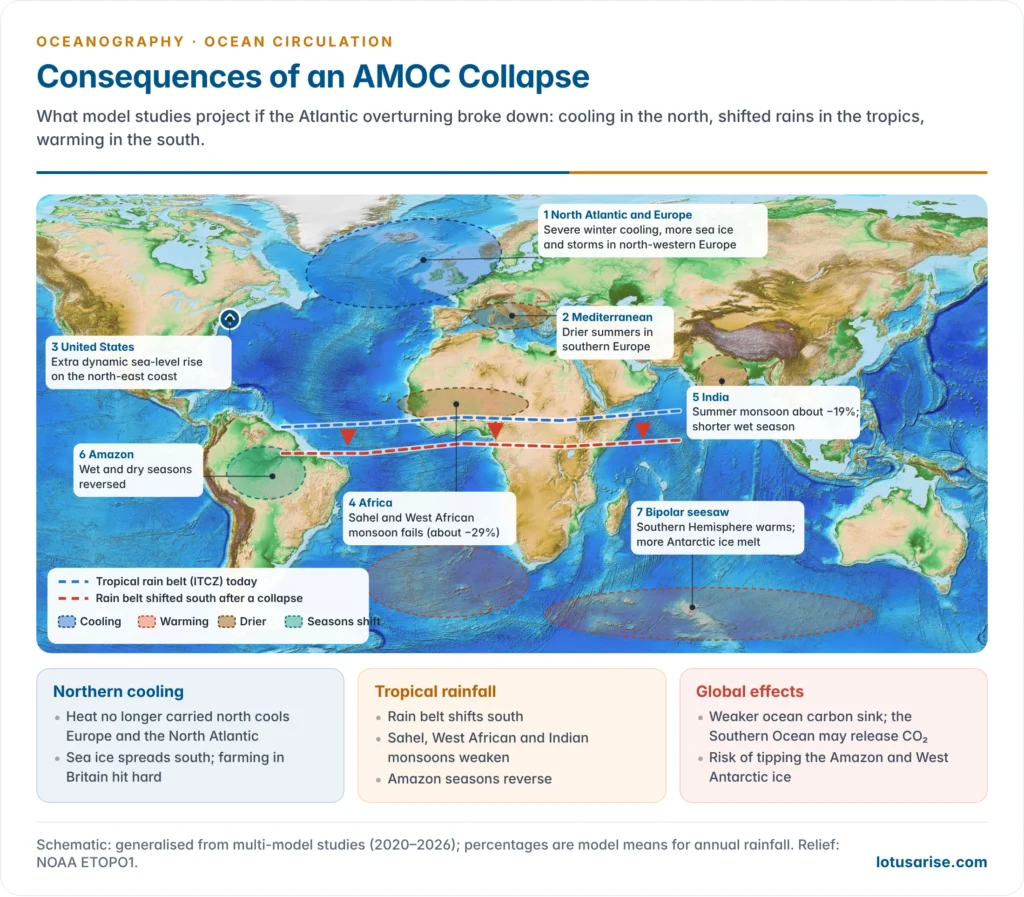
- The global temperature effect is small, but the regional effects are large. The tropics would keep the heat no longer carried north, so the Northern Hemisphere would cool and the Southern Hemisphere warm.
- North-western Europe:
- Winters would turn much colder, by 10–30 °C in northern Europe in one model (2024), with extreme cold of about −20 °C in London and −48 °C in Oslo under medium emissions (2025).
- Sea ice would spread further south. Storms and summer drought, especially in southern Europe, are expected to increase.
- Losses in arable farming in Britain could exceed those from warming alone (2020).
- Sea level:
- A slower Gulf Stream lets water pile up along the north-eastern US coast, adding dynamic sea-level rise on top of the global rise.
- The 2009–10 AMOC dip coincided with a jump of about 128 mm in sea level north of New York in two years.
- The tropical rain belt (ITCZ) would shift south:
- The West African and Sahel monsoon would fail most severely, with annual rainfall falling by about 29% in a four-model comparison (2024).
- The Indian summer monsoon would lose about 19% of its rainfall, with a shorter wet season. This threatens Kharif agriculture, water supply and food security in India.
- The East Asian monsoon would weaken slightly, while the Amazon would see its wet and dry seasons reversed.
- Carbon and ecosystems:
- Weaker sinking would slow the ocean’s uptake of CO₂. A 2026 study found that a collapse could also turn the Southern Ocean into a carbon source, adding about 0.2 °C of global warming.
- North Atlantic plankton and fisheries would be disrupted, and less oxygen would reach the deep ocean.
- Cascading tipping points: the AMOC interacts strongly with other tipping elements. Its collapse could hasten the loss of the Amazon rainforest and of the West Antarctic ice sheet.
| Region | Likely change after a collapse | Main mechanism |
|---|---|---|
| North-western Europe | Severe winter cooling, more sea ice and storms, drier summers | Loss of northward ocean heat transport |
| US north-east coast | Extra sea-level rise | Weaker Gulf Stream lets the coastal sea surface rise |
| Sahel and West Africa | Sharp fall in monsoon rain | Southward shift of the ITCZ |
| India and South Asia | Weaker, shorter summer monsoon | Cooler northern Atlantic and a southward rain belt |
| Amazon and southern South America | Reversed wet and dry seasons; wetter south | Rain belt shifts south |
| Southern Hemisphere and Antarctica | Warming, more ice-shelf melt | Bipolar seesaw |
| Global | Weaker ocean carbon sink; small net cooling on top of warming | Less deep-water formation |
Previous Year Questions
2026Discuss the potential consequences of the collapse of the Atlantic Meridional Overturning Circulation (AMOC) for the world.2011“Temperature, salinity and density differences in ocean water are the prime causes of ocean water circulation.” Elaborate.2009Comment on marine heat budget and the oceanic circulation system.