Drainage Basin: Concept, Patterns, Morphometry and Evolution

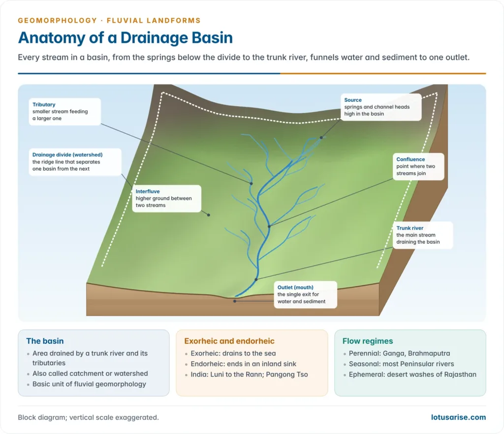
• A drainage basin is the area of land whose runoff drains to a single outlet on a stream or river; it is bounded by a drainage divide and holds a branching drainage network.
• Because its limits are fixed by relief, it carries both water and sediment, and it nests into ever larger basins, the drainage basin is the fundamental unit of fluvial geomorphology and hydrology.
• Its study has two sides: the genetic side (how streams originate and adjust to slope and structure: drainage systems, patterns, river capture and drainage evolution) and the quantitative side (morphometry: measurement of the network’s linear, areal and relief properties).

The Drainage Basin

Meaning and Related Terms

• Drainage basin (river basin, catchment): all the ground that supplies rain and meltwater to a given stream and its tributaries.
  • Water falling inside it leaves as evapotranspiration or through the basin mouth, after travelling as overland flow, throughflow or groundwater flow.
• Drainage divide (water divide): the line of higher ground, usually along ridge crests, separating the runoff of adjacent basins; it forms the basin perimeter.
  • The Western Ghats divide the short west-flowing rivers from the long east-flowing Peninsular rivers; the Vindhyas separate the Narmada from the Ganga system; the Ambala divide separates the Indus and Ganga systems.
• Watershed: strictly the divide line itself (British usage); in American and Indian planning usage, the whole small basin.
• Catchment area: the area draining to a chosen point such as a dam, lake or gauging station, not necessarily the river mouth.
• Drainage network: the master stream and all its tributaries, perennial, seasonal and ephemeral, down to rills and fingertip channels.
• Nested hierarchy: a large river basin is made of sub-basins, which are made of smaller watersheds and micro-watersheds, each with its own divide and outlet.
  • India-WRIS, using SRTM elevation data, delineates the country into 25 major river basins and 103 sub-basins; watershed programmes work at the micro-watershed level within this hierarchy.

Growth of the Basin Concept

• Pierre Perrault (1674) measured rainfall over the upper Seine basin and showed that only about one-sixth of the rainfall was enough to sustain the river’s annual flow, the first quantitative use of the basin as a unit.
• John Playfair (1802) observed that rivers carve their own valleys and that tributaries join the main stream at accordant levels, implying that the basin works as one integrated system (Playfair’s Law).
• William Morris Davis (1899) extended “the river” over its whole basin up to the divide: the channels are like the veins of a leaf, the basin is the whole leaf.
• Robert Elmer Horton (1932, 1945), an American hydraulic engineer, gave the first quantitative description of basin characteristics and, in 1945, treated the basin as a morphometric system governed by regular laws.
• Richard John Chorley (1969) called the basin the fundamental geomorphic unit: clearly bounded, available in a nested hierarchy of sizes, and an open system for which inputs and outputs can be measured.

Drainage Basin as an Open System

• In the systems framework of Richard Chorley and Barbara Kennedy (1971), the basin is an open system that exchanges both energy and matter with its surroundings.
  • Energy comes from the atmosphere (precipitation, solar radiation) and from within the Earth, since uplift, warping, folding and faulting give the relief whose potential energy erosion uses.
  • Energy and mass leave through evapotranspiration and the outflow of water, sediment and solutes at the basin mouth.

Component	Contents
Inputs	Rain, snow, meltwater; solar radiation; uplift supplying potential energy
Stores	Interception, surface, soil moisture, groundwater, channel storage, lakes
Transfers	Stemflow, infiltration, percolation, overland flow, throughflow, base flow, channel flow
Outputs	Evapotranspiration; discharge, sediment and solute yield at the mouth
Regulators	Slope, lithology, soil, vegetation, land use, climate

• An open system tends towards dynamic equilibrium: channel width, depth, gradient and drainage density adjust to the discharge and load supplied.
  • A disturbance (deforestation raising runoff, a dam trapping sediment) sets off readjustment through negative feedback until a new quasi-equilibrium is reached.
  • Where a threshold is crossed (gullying, avulsion), change is abrupt.

Drainage Basin Hydrological Cycle

• The basin hydrological cycle moves water from one input (precipitation) through a chain of stores to two outputs.

Store	Receives	Loses by
Interception (canopy)	Rain on vegetation	Evaporation; stemflow and drip to the ground
Surface	Throughfall, stemflow, direct rain	Overland flow, evaporation, infiltration
Soil moisture	Infiltration, capillary rise	Evapotranspiration, throughflow and interflow, percolation
Groundwater	Percolation	Base flow, capillary rise, deep transfer
Channel	Overland flow, throughflow, base flow	Channel runoff at the mouth

• Outputs: evapotranspiration from the upper stores and channel runoff from the channel store.
• Almost every basin is now modified by people: urban surfaces cut infiltration and sharpen flood peaks, irrigation and groundwater pumping cut base flow, and reservoirs store water and sediment.

Drainage Systems and River Capture

Genetic Basis

• A drainage system is the origin and development of streams through time in relation to slope and structure; a drainage pattern is the spatial arrangement (geometry) of the network as seen on a map.
  • The descriptive approach studies form and pattern; the genetic approach studies the evolution of streams in relation to tectonics, lithology and structure.
• Two factors control a drainage system: the nature and slope of the initial surface, and the geological structure (folds, faults, joints, dip and strike, rock type).
• By their adjustment to slope and structure, streams fall into sequent (concordant) streams, which follow the regional slope and adjust to structure, and discordant streams, which cut across structure.

Sequent (Concordant) Streams

Consequent Streams

• Consequent streams are the first streams to form on a new surface and follow its initial slope; in dipping strata they are also called dip streams.
  • The longest and most active is the master consequent.
  • In folded terrain, longitudinal consequents occupy synclinal troughs and lateral consequents run down the flanks of anticlines, joining them nearly at right angles.
• Ideal settings: newly emerged coastal plains (parallel consequents), domes and volcanic cones (radial consequents).
• Indian example: most streams crossing the Konkan and Coromandel coastal plains are consequents.

Subsequent Streams

• Subsequent streams develop after the consequents, usually as their tributaries, and grow headward along belts of weakness: soft strata, faults, joints and shatter zones, typically along the strike.
  • Sidney William Wooldridge and Richard Stanley Morgan treated all first-generation tributaries of consequents as subsequent, since they arise after the consequent valleys are incised and then seek out weak belts; the term marks a relation to structure more than an order in time.
• Indian example: in the Dehra Dun valley, the Asan (to the Yamuna) and the Song (to the Ganga) are strike subsequents of the master consequents, the Yamuna and the Ganga.

Obsequent Streams

• Obsequent streams flow opposite to the master consequent, usually down the scarp face of a cuesta or the back slope of a ridge, and join a subsequent.
  • They too follow a local slope, so they are consequent in the broad sense.
• Indian example: streams from the northern slopes of the Mahabharat Range in Nepal flow north into the west–east Sun Kosi, against the southward course of the Himalayan master streams; streams from the northern slopes of the Siwaliks behave in the same way.

Resequent Streams

• Resequent streams flow in the same direction as the original consequents but at a lower level, having developed later in the erosional history.
• They arise through inversion of relief in folded rocks.
  • During the first cycle, the stretched and jointed anticlinal crests erode faster, so anticlinal ridges become anticlinal valleys and the resistant synclinal cores stand up as synclinal ridges.
  • When a new cycle begins on the lowered surface, streams re-excavate the synclines and flow like the original longitudinal consequents, but hundreds of metres below the initial surface.

Insequent Streams

• Insequent streams show no evident control by slope or structure: they develop by random headward growth on rocks of uniform resistance or on horizontal beds.
  • They build the dendritic pattern and dominate plains and flat-lying plateaus, such as the Deccan lava country.
• Wider usage: the term insequent (inconsequent) is also used for every stream not adjusted to regional slope and structure, which groups antecedent and superimposed streams as insequent.
  • In the stricter usage, those are discordant streams, and insequent is kept for networks with no evident structural control.

Discordant (Inconsequent) Streams

Antecedent Streams

• An antecedent stream existed before an upland rose across its course and kept that course by cutting down as fast as the land rose.
• Conditions:
  • Slow and steady uplift: if uplift outpaces incision, the river is ponded, deflected or dismembered.
  • Local uplift across the course (a rising ridge or range), not broad regional upwarping.
  • A river with enough discharge and gradient to keep incising.
• Mechanism: uplift rejuvenates the river; while incision matches uplift, the bed level stays nearly constant and the course holds.
• Landforms:
  • Deep, narrow gorges with near-vertical, often convex walls across the rising range.
  • Hanging tributary valleys, because tributaries cannot incise as fast as the master stream.
  • Flights of river terraces recording pulses of uplift.
• Himalayan examples (the Himalaya rose in pulses through the Cenozoic); the Indus gorge near Nanga Parbat is several kilometres deep.

Antecedent to	Rivers
Great Himalaya, Lesser Himalaya and Siwaliks	Indus, Sutlej, Karnali (Ghaghra), Gandak, Arun (Kosi), Brahmaputra
Lesser Himalaya and Siwaliks	Jhelum, Ravi, Yamuna, Ramganga
Siwaliks only	Rapti, Kamla, Gola

• Arun: Lawrence Rickard Wager (1937) made the Arun the classic case. It flows east along the structural grain in Tibet, turns abruptly south and crosses the Himalaya in entrenched gorges with terraces on both sides, fitting sustained incision during uplift.
• Evaluation:
  • The rates of uplift and incision in the past cannot be measured directly, so antecedence is often inferred rather than proved.
  • An alternative view holds that consequents on the steep southern slope eroded headward, shifted the divide north and captured north-slope streams; the southward bend of the Arun is read by some as a capture elbow.
  • The current view treats trans-Himalayan courses as the product of antecedence combined with headward capture and divide migration, with focused erosion in the gorges feeding back on local uplift.

Superimposed Streams

• A superimposed (epigenetic) stream established its course on a younger cover lying unconformably over older rocks of different structure, then cut down through the cover and kept its course on the buried structure.
  • John Wesley Powell (1875) named both antecedent and superimposed valleys during his survey of the Colorado; W J McGee (1888) used “superposed” for the same process.
• Stages:
  1. A consequent develops on the flat cover (horizontal sediments or lava).
  2. The river incises, and the cover is gradually stripped.
  3. The river meets the older structure (folds, domes, batholiths) and cuts across ridges it would never have crossed had that structure been exposed first.
• Indian examples:
  • Many rivers of the Deccan lava region began on the lava surface formed in the late Cretaceous and early Palaeogene and were later superimposed on older rocks as the lava was stripped.
  • The Subarnarekha crosses the Dalma hills west of Chandil in the south-eastern Chotanagpur plateau; the Damodar is also treated as superimposed on the Chotanagpur structures.
  • The Son cuts twice across the Khainjua ridges of Lower Vindhyan quartzitic sandstone in the southern Rewa plateau, near Deoland and again below its confluence with the Banas.
• Why the Son is superimposed, not antecedent: the ridges were folded before the Upper Vindhyans were laid down, with no later local uplift; laterite north of the Kaimur scarp points to a former Deccan lava cover on which the Son took its course before being lowered onto the ridges.

Basis	Antecedent	Superimposed
Relative age	River older than the uplift	River older than the exposed structure
Cause of discordance	Uplift across the course	Removal of an unconformable cover
Tectonics needed	Yes, slow local uplift	No
Typical forms	Gorges, hanging valleys, terraces	Water gaps across ridges, cover remnants
Examples	Indus, Sutlej, Arun, Brahmaputra	Subarnarekha (Dalma), Son (Khainjua)

Twin-River (Subterranean) System

• A twin-river system is a pair of flows at two levels in the same region, one on the surface and one deep below it, following the same direction and regional gradient; it is a rare geological case.
• Amazon–Hamza pair: in 2011 a team led by the Indian-born geophysicist Valiya Mannathal Hamza of Brazil’s National Observatory inferred, from temperature records of 241 abandoned oil wells, a slow west-to-east flow of groundwater about 4 km beneath the Amazon, named the Hamza “river”.
  • It runs about 6,000 km from the Andean foothills to the Atlantic, like the Amazon above it.
  • It is far wider (about 200–400 km) than the Amazon but moves at less than 1 mm a second, slower than a glacier, with a discharge of roughly 3,000 m³/s, about 3% of the Amazon’s.
  • Water infiltrates through permeable sedimentary rocks, and west–east faults serve as conduits to depth; the west-to-east slope of the basin, from the Andes to the Atlantic, guides both flows.
• The result is preliminary and contested: it is a deep, sluggish movement of groundwater through porous rock, not a river in the usual sense, and awaits independent confirmation.

River Capture

• River capture (stream piracy, stream diversion) is the diversion of part of one river’s course into another that is eroding more actively.
  • The captor (capturing) stream gains the water; the captured stream loses its headwaters.
  • It is most active in youth, through headward erosion, but continues in maturity and old age through lateral erosion and meander cut-offs.
• Much of the present Himalayan drainage is the outcome of progressive capture at different stages.

Conditions Favouring Capture

• The captor must erode faster than its neighbour, which happens with:
  • a steeper channel gradient and a deeper valley (lower local base level);
  • greater discharge and velocity, and a low sediment load leaving energy for erosion;
  • a narrow valley that concentrates flow;
  • softer rocks and higher rainfall on its side of the divide;
  • a shorter course to base level, so the divide slope facing it is steeper.

Evidence of Capture

Feature	Meaning
Elbow of capture	Sharp, often right-angled bend where the captured headwaters turn into the captor
Water gap	Gorge cut through a ridge by the captor’s headward erosion
Wind gap (col)	Dry, abandoned valley segment just below the elbow
Misfit (underfit) stream	Beheaded stream too small for its inherited valley
Beheaded stream	Lower course of the captured river, left without its headwaters
Barbed tributaries	Tributaries pointing upstream, recording reversed flow

• A tributary whose flow is reversed after capture is an inverted stream; the captor, with extra discharge, incises faster, while the beheaded stream’s erosion almost stops.

Types of Capture

Type	Process	Stage	Setting
Headward erosion	Captor extends its head across the divide and taps a neighbour	Youth	Mountains, escarpments
Lateral erosion (abstraction)	Larger parallel streams widen their valleys and consume smaller ones	Maturity	Coastal and sedimentary plains
Meander intersection	Meanders of adjacent streams erode laterally until they meet	Late maturity, old age	Alluvial plains

• Headward capture is the commonest: a tributary of the deeper-valleyed stream erodes back through the divide, cuts a water gap and diverts the neighbour’s tributary and upper course, leaving an elbow, a wind gap and a misfit lower valley.

Indian Examples

• Arun and the Tsangpo: the Arun has captured a southern tributary of the Tsangpo by headward erosion across the Himalayan crest.
• Dehra Dun: the divide between the Song (Ganga system) and the Asan (Yamuna system) is only a few metres wide; if the Song taps the Asan, part of the Yamuna headwaters could pass to the Ganga.
• Western Ghats: the divide between the headwaters of the west-flowing Savitri and the east-flowing Krishna near Mahabaleshwar is very narrow; the steep west-facing streams are extending eastward.
• Belan–Seoti: near Deoghat, south of Prayagraj, the Belan (a Tons tributary) captured the lower course of the Seoti by meander intersection, shifting their confluence about 6 km upstream and leaving the old Belan valley as a misfit palaeochannel.
• Ghaggar–Hakra: this palaeochannel lost its Himalayan feed as the Sutlej swung west to the Indus system and the Yamuna east to the Ganga; dating of its sediments shows the Sutlej abandoned it about 8,000 years ago, well before the Harappan urban phase.
• Current view: elevation models now show where divides are migrating; Sean Willett and colleagues (2014) showed that basins are continually reorganised by divide migration and capture, so capture is a normal, ongoing process.

Drainage Patterns

• A drainage pattern is the geometric arrangement of a stream network in plan; it reads out the slope, lithology, structure, tectonics, climate and denudation history beneath it.

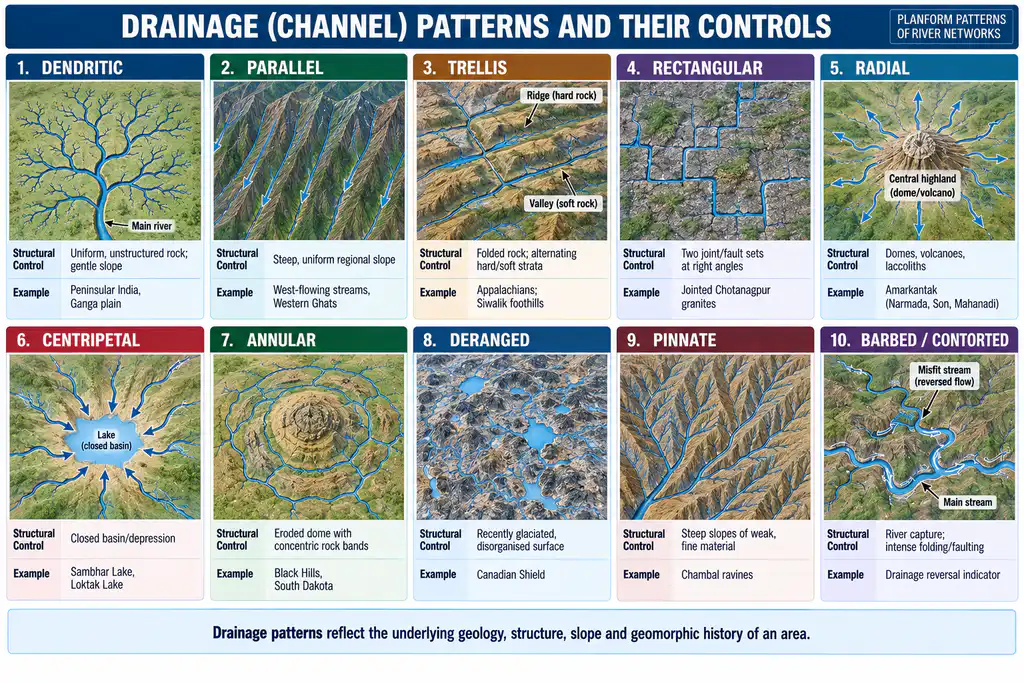
Pattern	Form	Main control	Examples
Dendritic	Tree-like, acute junctions	Uniform rock, gentle slope	Ganga plain, Deccan, Ranchi plateau
Parallel	Near-parallel streams	Uniform steep slope, new coastal plain	West-coast streams from the Western Ghats
Trellis	Main streams along strike, short tributaries at right angles	Folded alternating hard and soft beds	Appalachians; parts of Singhbhum
Rectangular	Right-angled bends in main and tributary streams	Two joint or fault sets	Jointed granite-gneiss of Chotanagpur
Radial	Streams diverge from a centre	Dome, volcano, isolated upland	Amarkantak; Sri Lanka; Parasnath
Centripetal	Streams converge on a centre	Basin or depression	Loktak, Sambhar, Kathmandu valley
Annular	Concentric subsequent arcs	Dissected dome with ring-like beds	Black Hills (USA), Weald (England)
Pinnate	Closely spaced short tributaries at acute angles	Narrow valley between steep ridges; fine weak material	Upper Son and Narmada; Chambal ravines
Herringbone	Rib-like tributaries at near right angles	Broad longitudinal valley between parallel ridges	Upper Jhelum, Vale of Kashmir
Barbed	Tributaries point upstream with hooked junctions	River capture, flow reversal	Rare; capture zones
Deranged	Disorganised streams, lakes and swamps	Recently glaciated surface	Canadian Shield, Finland
Contorted	Sharp irregular bends	Intensely folded and faulted metamorphics	Old orogenic belts

Dendritic

• The commonest pattern: tributaries of many orders join the trunk at acute angles like the branches of a tree.
• Controls: homogeneous lithology, horizontal or gently dipping strata, low relief; it develops wherever structure exerts little control, from plains to mountains.
• Development:
  • It starts open (few, widely spaced streams), becomes close as tributaries multiply by headward erosion, and in late stages is simplified as smaller streams are absorbed by capture (abstraction).
  • On flat, impermeable surfaces the network spreads in both length and width; on steeper slopes it becomes elongated.
• Indian examples: the Ganga plain, the peneplains of the Mahanadi, Godavari, Krishna and Cauvery basins, the Panna, Bhander and Rewa plateaus and the Ranchi plateau.

Parallel

• Streams run roughly parallel with few tributaries, down a uniform, steep regional slope: newly emerged coastal plains, tilted blocks, cuesta back slopes.
• It is essentially an initial pattern that tends to become subparallel or dendritic with time.
• Indian example: the short, swift streams from the western face of the Western Ghats to the Arabian Sea; parallel consequents also cross the Eastern Coastal Plains.

Trellis

• Longitudinal (master) consequents occupy synclinal or strike valleys, and short lateral consequents and subsequents join them at right angles from the flanking ridges.
• Controls: simple folds with parallel anticlinal ridges and synclinal valleys, or cuesta country with alternating resistant and weak beds.
• Trellis vs rectangular: in trellis, junction angles follow strike and dip and streams are closely spaced; in rectangular, they follow joints and faults and streams are widely spaced.
• Examples: the Appalachian Ridge and Valley (classic case); trellis-like networks in folded parts of Singhbhum and the Siwalik–Lesser Himalayan belt.

Rectangular

• Main streams and tributaries make abrupt right-angled bends.
• Controls: rock of fairly uniform resistance cut by two sets of joints or faults at right angles; weathering opens the joints into clefts that rills and then channels follow.

Radial (Centrifugal)

• Streams diverge in all directions from a central high, like spokes of a wheel; being slope-following, they are consequents.
• Controls: domes, volcanic cones, laccoliths and batholiths, residual hills, mesas and isolated uplands.
• Indian examples:
  • Amarkantak plateau, source of the Narmada, Son and Johilla.
  • The upland south-west of Ranchi, from which the South Koel, Subarnarekha, Kanchi and Karo radiate; Hazaribagh plateau, Parasnath hill and Mount Abu.
  • The Rohtas plateau, where the Karamnasa and Durgawati flow west and north while Son tributaries flow south.
• At the macro scale the whole drainage of Sri Lanka is radial from its central highlands.

Centripetal (Inland)

• The reverse of radial: streams converge on a central depression, basin or crater lake rather than draining to the sea.
• Examples: Loktak Lake (Manipur), Sambhar Lake (Rajasthan) and the Bagmati headstreams in the tectonic Kathmandu valley.

Annular (Circular)

• Tributaries run in concentric arcs around a mature, dissected dome whose truncated beds form rings of hard and soft rock.
  • The master consequents radiate from the dome’s top; subsequents occupy the soft rings and join them, so the pattern begins radial and becomes annular, a special case of trellis.

Pinnate and Herringbone

• Pinnate: short, closely spaced tributaries from steep valley sides join a longitudinal master stream at acute angles, like the veins of a leaf or a feather.
  • It forms in narrow valleys flanked by steep ranges (upper Son and Narmada) and on steep slopes of fine, easily eroded material (gullied Chambal ravines).
• Herringbone (rib) pattern: in a broad longitudinal valley between parallel ridges, straight tributaries from the steep slopes join the longitudinal consequent almost at right angles, like the bones of a herring.
  • The upper Jhelum in the Vale of Kashmir and rivers in east–west Himalayan trenches show it.

Barbed, Deranged and Contorted

• Barbed: tributaries join the main stream with a hook-shaped bend pointing upstream, usually because the main stream’s flow was reversed by capture; it is rare and is itself an evidence of capture.
• Deranged (indeterminate): an unintegrated network of streams, lakes and swamps on recently glaciated ground, where ice erased the old drainage; with time it integrates into an ordered pattern.
• Contorted: sharply bent, irregular streams on intensely folded and faulted metamorphic rocks, where foliation and jointing exert local control.

Drainage Basin Morphometry

Meaning and Development

• Morphometry is the measurement and mathematical analysis of the configuration of the Earth’s surface and of the shape and dimensions of its landforms; for a basin it covers area, altitude, volume, slope, profiles and network properties.
  • Relief morphometry: hypsometric, clinographic and altimetric curves and profiles.
  • Fluvial (basin) morphometry: the linear, areal and relief aspects of a fluvially eroded basin.
• Phases:
  • Nineteenth and early twentieth century: heights, volumes, slopes and erosion surfaces measured from maps.
  • From Horton (1945): intensive quantitative study of small drainage basins, carried forward by Arthur Newell Strahler, Stanley Alfred Schumm, Mark A. Melton, Richard Chorley and others in the 1950s–60s.
  • Today: basins and networks are extracted automatically from digital elevation models (SRTM, ISRO’s CartoDEM) in GIS, with satellite imagery replacing much manual map work.

Linear Aspects

• The linear aspects treat the network as a graph: junctions are nodes and stream segments are links, which are ordered, counted and measured.

Stream Ordering

• Stream order is a measure of the position of a stream in the hierarchy of tributaries (Luna Bergere Leopold, M. Gordon Wolman and John P. Miller, 1964).

Scheme	Rule	Merit	Limitation
Harry Gravelius (1914)	Trunk stream is order 1; its tributaries 2, theirs 3, up to the fingertips	First attempt	Subjective at each fork; order unrelated to size
Robert Horton (1945)	Fingertips are order 1; two equal orders make the next; then one branch is renumbered headward so the trunk carries the highest order to the source	Trunk is the longest line	Tedious reclassification; some fingertips upgraded
Arthur Strahler (1952)	As Horton, but no renumbering; a lower order joining a higher one leaves it unchanged	Simple, objective; standard today	Lower-order inflows ignored
Adrian Scheidegger (1965)	Consistent ordering on a ratio scale from link indices (G = log₂ of twice the magnitude)	Better reflects flow magnitude	Laborious; no bifurcation ratio
Ronald Shreve (1966)	Each exterior link has magnitude 1; magnitudes add at every junction	Every tributary counts; tracks discharge	Not an ordinal hierarchy

• Strahler’s segment method is the standard for morphometric laws: it keeps ordering ordinal and gives the same basin order as Horton’s.
  • Its weakness: many lower-order inflows do not raise the trunk’s order, yet adding a single first-order segment high in the basin can.

Bifurcation Ratio and the Law of Stream Numbers

• Bifurcation ratio (Rb) = Nu / Nu+1, the number of segments of one order divided by the number of the next higher order.
• Horton’s law of stream numbers (1945): the numbers of segments of successively lower orders form an inverse geometric series, beginning with one segment of the highest order and increasing by a constant Rb.
  • A fifth-order basin with Rb = 4 has 1, 4, 16, 64 and 256 segments, 341 in all; on semi-log paper, stream number against order gives a straight line.
• Values:
  • Rb usually lies between 3 and 5 where structure does not distort the network.
  • Horton expected about 2 on flat or rolling land and 3–4 in dissected uplands; studies of Chotanagpur, Rewa and Bhander basins found 3–5 on both, with dissected basins only slightly higher.
  • High Rb (much above 5) marks strong structural control and elongated basins.
• Behaviour: Rb tends to fall slightly with increasing order and varies little from region to region, much of the variation being chance.
• Hydrological meaning: a low Rb (rounded basin, tributaries meeting near together) gives a high, sharp flood peak; a high Rb (elongated basin) spreads arrivals and gives a lower, longer peak.

Stream Length and the Law of Stream Lengths

• Mean stream length (Lu) = total length of segments of an order ÷ their number; length ratio (RL) = Lu / Lu−1.
  • Total length per order falls with increasing order, while mean length rises.
• Horton’s law of stream lengths (1945): cumulative mean lengths of successive orders form a direct geometric series starting from the mean first-order length, with a constant RL.
  • Real basins rarely hold RL constant, so the law is a statistical tendency; gully networks near Prayagraj fit it closely.

Length of Overland Flow

• Length of overland flow (Lg) is the mean horizontal distance water travels from the divide to a channel before concentrating; it is about half the reciprocal of drainage density (Lg ≈ 1/2Dd).
• It is longest in youth and shortest in late youth and early maturity, when the network is densest.
  • Rainfall intensity, infiltration, soil and vegetation also control it, so stage should not be read from it alone.

Sinuosity and Junction Angles

• Sinuosity measures the departure of a stream’s actual path from a straight line (observed ÷ expected length).
  • Stanley Schumm (1963) classed channels as straight (1.0), transitional, regular, irregular and tortuous; J. E. Mueller (1968) separated hydraulic from topographic sinuosity, the topographic share falling as relief controls weaken with basin age.
• Junction (entrance) angles tend to widen as the order of the receiving stream rises.
  • Where valley-side slopes are steep relative to the master stream, tributaries enter nearly at right angles; where the two gradients are similar, they enter at small angles; entrance angles are smaller in mature basins than in youthful ones (Schumm, 1956).

Areal Aspects

Basin Area, Perimeter and Shape

• Basin area correlates with almost every other basin property, which led H. W. Anderson (1957) to call it the “devil’s own variable”; it is cumulative, each order’s area including all the lower-order basins and inter-basin areas within it.
• Basin perimeter rises with the square root of area, and channel length with both, because first-order streams notch back the divides and enlarge area, length and perimeter together.
• Shape is usually summarised by dimensionless indices.

Index	Formula	Range and meaning
Form factor, Robert Horton (1932)	Rf = A / L²	0 (elongated) to about 0.79 (circle)
Circularity ratio, V. C. Miller (1953)	Rc = 4πA / P²	0 (line) to 1 (circle)
Elongation ratio, Stanley Schumm (1956)	Re = (2/L)√(A/π)	0 (elongated) to 1 (circle)
Compactness coefficient, Gravelius (1914)	Cc = P / 2√(πA)	1 for a circle, larger when irregular
Lemniscate ratio, Chorley, Malm and Pogorzelski (1957)	k = πL² / 4A	Larger value, more elongated

• Hydrological meaning: runoff from a circular basin reaches the outlet almost together and gives a sharp, high flood peak; an elongated basin gives a lower, delayed and prolonged peak.
• Shape and stage: basins are expected to grow rounder (pear-shaped) with age, but structure usually dominates; a basin squeezed between parallel ridges stays elongated even in old age.

Laws of Basin Area and Allometric Growth

• Area ratio is the ratio of mean basin areas of successive orders.
• Law of basin areas (Schumm, 1956, restated by Strahler): mean basin areas of successive orders form a geometric series beginning with the mean first-order area and increasing by a constant area ratio.
  • It holds where the area ratio is fairly stable and weakens where it varies.
• Law of allometric growth: borrowed from biology, where an organ grows as a constant fraction of the whole organism’s growth.
  • Marie Morisawa, Michael Woldenberg and Strahler showed that cumulative mean stream length and mean basin area plot as a straight line on log–log paper, so network and basin grow in fixed proportion.

Drainage Density, Stream Frequency and Texture

• Drainage density (Dd) = ΣL / A, total stream length per unit area (Horton, 1945); stream frequency (Fs) = ΣN / A, number of segments per unit area (Horton, 1932).
  • Both are mapped over grid squares (usually 1 km²) and shown as isopleths or choropleths, because a single basin value hides internal variation.
  • Quicker estimates count stream crossings along grid edges and diagonals; this spacing measure correlates above 0.9 with Dd in Chotanagpur and Aravalli basins.
• Constant of channel maintenance (C = 1/Dd) (Schumm, 1956): the area needed to sustain one unit length of channel.
• Drainage texture is the relative spacing of drainage lines (coarse, medium, fine), set by Dd and stream frequency together.

Factor	High Dd (fine texture)	Low Dd (coarse texture)
Rock and soil	Impermeable clays, shales, weak rocks	Permeable sandstone, limestone, jointed granite
Vegetation	Sparse	Dense forest or grass
Rainfall	Intense storms, semi-arid regime	Gentle rain, high infiltration
Relief	Steep, high relative relief	Gentle, low relief
Indian case	Chambal ravines, Siwalik badlands	Less dissected Deccan and Malwa plateau surfaces

• High Dd means short overland flow paths, quick runoff and high sediment yield; low Dd means more infiltration and groundwater recharge, which is why low-Dd tracts are favoured for well siting.

Relief Aspects

Hypsometric Analysis

• Hypsometry relates altitude to area to judge the degree of dissection and the stage of erosion.
  • Area–height curve: area between successive contours against height.
  • Hypsometric curve: cumulative percentage of area above each contour against height.
  • Neither shows the real profile, and breaks of slope are hidden.
• Percentage hypsometric curve (Strahler, 1952): relative height (h/H) against relative area (a/A), making basins of any size comparable.
  • Hypsometric integral (HI): the area under the curve, the share of the original rock mass still unconsumed; the area above it is the erosion integral.
  • HI above 0.6: youthful, disequilibrium stage (convex curve); 0.35–0.6: mature, equilibrium stage (S-shaped); below 0.35: monadnock (old) stage (concave).
  • The low value lasts only while monadnocks remain; once they go, HI returns to about 0.4–0.6, so it needs field checks.

Slope and Clinographic Analysis

• Clinographic curves plot the average slope between successive contours against height and, unlike hypsometric curves, reveal breaks of slope.
  • Methods include those of Sebastian Finsterwalder, J. Hanson-Lowe (1935), Strahler (mean inter-contour width), R. De Smet and Moseley’s slope–height curve.
• Average slope is mapped by Chester Keeler Wentworth’s (1930) method: contour crossings are counted along grid lines, converted to slope angles and grouped into classes from level (0–2°) to very steep (above 30°); it cannot handle cliffs.

Altimetric Analysis

• Altimetric frequency analysis counts spot heights, summits, benches and shoulders by height class; peaks in the frequency curve point to old erosion surfaces.
  • Henri Baulig used it to trace flats left by falling base levels.
  • Warping can also produce summit concordance, so peaks must be checked in the field.

Relief Indices

Index	Definition	Use
Relative (available) relief, Waldo S. Glock (1932)	Highest minus lowest point in a grid cell or basin	Degree of dissection
Relief ratio, Stanley Schumm (1956)	Basin relief ÷ basin length	Overall steepness; sediment yield
Ruggedness number, Arthur Strahler (1958)	Basin relief × drainage density	Steep and densely dissected basins
Dissection index, Dov Nir (1957)	Relative relief ÷ absolute relief (0 to 1)	Stage: higher values, more youthful
Channel slope, Robert Horton (1945)	Vertical drop ÷ length per order	Law of channel slopes

• Law of channel slopes (Horton, 1945): mean channel slope decreases with increasing order in an inverse geometric series; gullies near Prayagraj fit it almost perfectly.
• A high ruggedness number marks basins that are both steep and finely dissected, the combination most prone to flash floods and debris flows.

Profiles

• Longitudinal profiles show knickpoints, heads of rejuvenation that reveal polycyclic development.
• Terrain profiles: serial and superimposed profiles pick out planation levels; projected profiles show the landscape as seen from above; composite profiles trace the skyline of summits.
  • Superimposed profiles of the Belan basin show four surfaces: the Kaimur, Panna, Rewa and Trans-Yamuna–Ganga surfaces.

Evaluation of Morphometry

• Strengths: precise, comparable measures; objective description of stage and dissection; direct links to runoff, flood peaks and sediment yield.
• Criticisms:
  • Albrecht Penck (1894) warned that complex polycyclic landforms are hard to measure accurately; Alfred Hettner (1921) held that numbers cannot give a genetic explanation; Wooldridge (1958) doubted whether much geomorphic data needed or allowed quantification.
  • Ronald Shreve (1966) showed that topologically random networks obey Horton’s laws, and James W. Kirchner (1993) argued the laws are almost statistically inevitable, so fitting them reveals little about process.
  • Values of Dd, stream number and order depend on map scale, DEM resolution and where channel heads are drawn, so basins must be compared at the same scale.
• Current view: morphometry is most useful when tied to process, as in hydrological modelling, sediment budgets and tectonic geomorphology (hypsometry and channel steepness used to detect active uplift).

Applications

• Watershed prioritisation: Dd, stream frequency, Rb, shape and relief indices rank sub-watersheds for soil and water conservation, check dams and afforestation under programmes such as the Watershed Development Component of PMKSY.
• Flood and hazard assessment: basin shape, Dd and ruggedness drive the flood hydrograph; the steep, finely dissected first-order catchments above Mundakkai and Chooralmala in Wayanad, where debris flows on 30 July 2024 killed more than 200 people, show the hazard of high-relief, high-density basins in intense rain.
• Reservoir and groundwater planning: relief ratio and Dd indicate sediment yield and silting rates; low-Dd, gentle zones indicate better recharge.

Evolution of Drainage

• Initiation: when a surface emerges or is uplifted, consequents follow its initial slope and the pattern is parallel or radial.
• Waldo S. Glock (1931) described network growth in five stages.

Stage	What happens
Initiation	A few widely spaced channels appear
Elongation	Channels lengthen by headward erosion
Elaboration	Tributaries of successive orders multiply
Maximum extension	Drainage density and stream number peak
Abstraction (integration)	Capture and lateral erosion absorb small streams; the network simplifies

• Horton (1945) explained the start: overland flow erodes only beyond a critical distance from the divide (a belt of no erosion near the crest); below it rills form, the deeper ones capture their neighbours (micropiracy), and cross-grading turns the surviving rills into a branching network.
• Adjustment to structure: subsequents grow along weak belts and capture consequents, so an initially slope-guided network becomes adjusted to structure, as Davis (1889) showed for the rivers of Pennsylvania; resequents and obsequents appear as denudation proceeds.
• Stage in the Davisian cycle:

Stage	Network	Divides and relief	Indices
Youth	Few tributaries, lakes, falls, gorges	Broad, ill-drained divides	High HI, long overland flow
Maturity	Fully integrated, graded	Sharp divides, maximum relief	Maximum Dd
Old age	Sluggish meandering trunks on a peneplain	Low relief, monadnocks	Low HI, Dd reduced by abstraction

• Interruptions: uplift rejuvenates the network; tilting reverses or diverts it; glaciation deranges it; lava floods bury it and prepare it for superimposition.
• Indian drainage evolution:
  • Himalaya: the trans-Himalayan rivers are read as antecedent, modified by headward capture of Tibetan drainage. The Indobrahm (Siwalik River) hypothesis of Edwin Hall Pascoe (1919) and Guy Ellcock Pilgrim (1919) proposed a single west-flowing river along the Himalayan foot, later dismembered into the Indus, Ganga and Brahmaputra; it is now largely discounted, since Siwalik sediments were laid by separate transverse rivers building fans.
  • Peninsula: the Western Ghats divide and an eastward tilt send most rivers to the Bay of Bengal; the Narmada and Tapi flow west along faulted rift troughs; rivers of the lava country and Chotanagpur show superimposition, and the Ghats escarpment shows active headward capture.
• Current view: networks are dynamic; divides migrate and captures reorganise basins continually, so the classical sequence of stages is a useful ideal, not a fixed path.