- The New Economic Geography (NEG) is a branch of spatial economics that explains why economic activity concentrates in a few places. It accounts for the rise of agglomerations, industrial cores and lagging peripheries.
- It was launched by Paul Krugman in “Increasing Returns and Economic Geography” (Journal of Political Economy, 1991) and Geography and Trade (1991).
- Krugman received the Nobel Prize in Economics in 2008 for his analysis of trade patterns and the location of economic activity.
- Its core claim: increasing returns, transport costs and the mobility of firms and workers together produce cumulative, self-reinforcing concentration, even between regions that start out alike.
Origin and Meaning

From Spaceless Economics to Geographical Economics
- Mainstream economics long treated geography as irrelevant. It studied general principles of how economies work, without space.
- The shift came in the early 1990s, when Krugman applied modern trade theory and formal modelling to spatial questions. This approach integrated location into mainstream economic analysis.
- Intellectual roots:
- Alfred Marshall’s (1890) external economies of industrial districts.
- Gunnar Myrdal’s (1957) cumulative causation and Albert Hirschman’s linkages.
- Avinash Dixit and Joseph Stiglitz’s (1977) model of monopolistic competition, which made increasing returns tractable in formal models.
- Paul Samuelson’s “iceberg” representation of transport costs.
- The name is disputed. Many economic geographers prefer the term “geographical economics”.
- They argue that Krugman’s approach reorients economics rather than continuing geographical thought, the tradition carried by the other major theoretical perspectives in economic geography.
- The field has since grown fast. Economists now use mathematical models to study uneven development, industrial location and urbanisation.
- The Spatial Economy (Masahisa Fujita, Paul Krugman and Anthony Venables, 1999) set out its standard framework.
Definition
- Masahisa Fujita and Tomoya Mori (2005): the New Economic Geography is a new branch of spatial economics that aims to explain the formation of a large variety of economic agglomerations in geographical space.
- It works within a general-equilibrium framework. All markets and locations are solved together, which gives a systemic analysis of the spatial economy.
Key Characteristics
- General-equilibrium modelling:
- NEG models the whole spatial economy at once (consumers, firms, workers, regions), rather than one firm or one market in isolation.
- Increasing returns and indivisibilities:
- Production has increasing returns to scale at the level of the plant or firm.
- Without them, every household would produce everything it needs (“backyard capitalism“) and there would be no reason to concentrate.
- Increasing returns imply imperfect (monopolistic) competition and large-scale production.
- Transport costs:
- These create spatial friction and give location its significance.
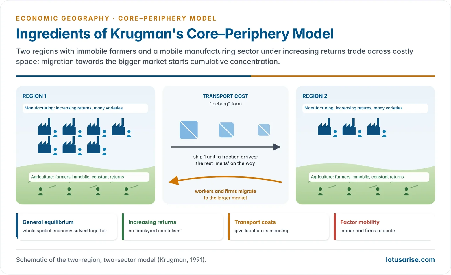
- They are usually modelled as “iceberg” costs: a fraction of each good “melts away” in transit.
- Locational movement of productive factors:
- The mobility of labour (as workers and consumers) and of firms is critical to the formation of agglomerations.
The Core–Periphery Model
Set-up
- Two regions, initially identical.
- Two sectors:
- Agriculture: constant returns, a homogeneous good and immobile farmers. This sector anchors demand in both regions.
- Manufacturing: increasing returns, many differentiated varieties and mobile workers.
- Transport costs apply to manufactured goods shipped between regions.
Cumulative Causation
- The model shows how a core, a hub of concentrated economic activity, emerges alongside a lagging periphery through three interacting forces:
- increasing returns at the firm level,
- transport costs that affect the mobility of goods,
- mobility of factors, especially labour and capital.
- Backward linkage (market-size effect): firms prefer the region with the larger market, to save transport costs on sales.
- Forward linkage (cost-of-living effect): workers prefer the region where more varieties are produced locally, because goods there are cheaper. Their migration enlarges the market further.
- The result is circular and cumulative causation:
- Small initial differences in cost, market size or history can tip the economy into full concentration.
- Over time the core becomes a magnet for labour, investment, infrastructure and innovation, and the gap with the periphery widens.
Conditions for a Core–Periphery Pattern
- Concentration is most likely when:
- Transport costs are sufficiently low, so it pays to concentrate production and serve distant markets from one place.
- Products are sufficiently differentiated, so firms gain from agglomeration without competing each other away.
- Manufactures take a large share of expenditure, so the mobile market is big enough to support scale economies.
- Home-market effect: a region with a larger market attracts a more than proportionate share of industry and becomes a net exporter of manufactures.
Centripetal and Centrifugal Forces
- Paul Krugman (1998) summarised the forces that pull activity together or push it apart.
| Centripetal (concentrating) forces | Centrifugal (dispersing) forces |
|---|---|
| Market-size effects: backward and forward linkages | Immobile factors: land, natural resources, part of the labour force |
| Thick labour markets | Land rents and housing costs |
| Pure external economies: knowledge spillovers | Pure external diseconomies: congestion, pollution |
- The balance between these forces decides whether activity concentrates or spreads out.

Break Point, Sustain Point and the “Tomahawk”
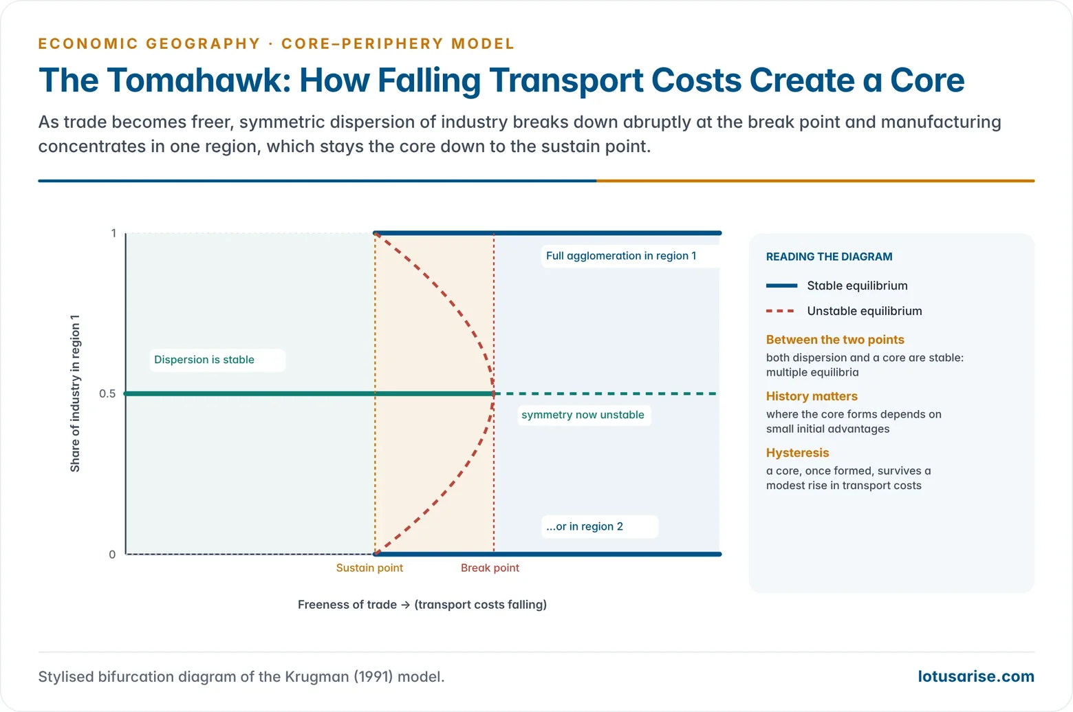
- As transport costs fall, the spatial economy changes abruptly, not smoothly.
- High transport costs: each region must supply itself, so industry stays dispersed.
- At the break point, the symmetric pattern becomes unstable. A small shock tips all industry into one region.
- At the sustain point, once formed, a core persists even if transport costs rise again a little.
- Plotted together, the stable outcomes form a “tomahawk” bifurcation diagram.
- The diagram shows multiple equilibria, path dependence and hysteresis: history matters.
- Later models add congestion and immobile workers, and give a bell-shaped relation.
- Concentration rises as trade costs fall from high to intermediate levels. At very low trade costs re-dispersion can follow, as firms seek cheaper labour and land.
Extensions of the Theory
Three Classes of NEG Models
| Class | Focus | Key idea |
|---|---|---|
| Core–periphery models | Two regions, mobile labour | Self-reinforcing concentration of manufacturing |
| Regional and urban system models | Number, size and spacing of cities | Emergence of a hierarchy of cities |
| International models | Countries, immobile labour, input–output links | Industrial clusters across borders; effect of trade on internal geography |
Regional and Urban Systems
- These models study the spatial coordination of agglomerations:
- the size of urban and regional agglomerations,
- their number within a region,
- their spacing across the landscape,
- inter-industry co-location: how different industries interact and locate together.
- The internal structure of each agglomeration, such as intra-urban land use, is simplified so as to focus on regional distribution.
- Krugman’s “racetrack economy” places locations evenly around a circle like positions on a racetrack. It shows how activity spreads or clusters among equidistant points, and how evenly spaced cities can emerge.
- As in the core–periphery model, factor mobility lets firms and workers relocate and so produces nested agglomerations: a hierarchy of cities that echoes central place theory.
International Trade
- In the international models, labour does not cross borders. Instead, input–output linkages between firms drive clustering of industries in particular countries.
- External market access reshapes internal geography.
- Paul Krugman and Raul Livas Elizondo (1996) showed that a closed economy favours a giant primate city such as Mexico City.
- Opening to foreign markets weakens the internal core–periphery pattern, as production moves towards border and port regions.
- This helps explain the growth of Mexico’s northern border states after trade liberalisation.
Frontiers in the Theory
- Original NEG models depended on special functional forms for utility, production and transport technology. Newer work relaxes these assumptions.
- New market-structure models:
- The Ottaviano–Tabuchi–Thisse (2002) model replaces the Dixit–Stiglitz framework. It allows pro-competitive effects and more flexible consumer preferences.
- Heterogeneous labour:
- Workers differ in innate skills and in migration behaviour (Tomoya Mori and Alessandro Turrini, 2005).
- Explaining spatial distribution therefore needs both market factors (demand, costs) and non-market factors (quality of life, preferences, institutions).
- Heterogeneous space: physical geography, borders and amenities are built in, replacing the uniform plain of early models.
- Heterogeneous firms: more productive firms sort into large markets.
- Spatial fragmentation of firms:
- Masahisa Fujita and Jacques-François Thisse (2006) modelled firms that split headquarters and plants between countries under monopolistic competition.
- This matters because fragmentation of production is a defining feature of globalisation.
- Growth and agglomeration: linking long-run accumulation and innovation to location is still an open frontier. It is analytically demanding.
- Quantitative spatial economics: recent models are calibrated to real data on trade, commuting and infrastructure. They are used to evaluate highways, railways and special economic zones.
Comparison, Applications and Evaluation
How NEG Differs from Traditional Location Theory
| Aspect | Traditional location theory (von Thünen, Weber, Lösch) | New Economic Geography |
|---|---|---|
| Analytical approach | Deductive, geometric, partial equilibrium | Mathematical general equilibrium |
| Space | Isotropic, uniform plain | Increasingly heterogeneous; outcomes from economic forces and geography |
| Returns to scale | Constant or diminishing | Increasing returns at the core |
| Transport cost | Static parameter to minimise | Iceberg costs that fall over time and reshape location |
| Market structure | Perfect competition | Imperfect (monopolistic) competition |
| Agglomeration | By-product of cost minimisation | Central, through circular and cumulative causation |
| Factor mobility | Restricted or ignored | Mobile labour and firms drive divergence |
| Policy relevance | Static optimal locations | Regional development, urbanisation, trade liberalisation, relocation |
- Weber’s least-cost model treats agglomeration as a deviation from the transport-cost optimum. NEG makes agglomeration the central outcome and explains it endogenously.
Applications and Policy
- World Development Report 2009 (Reshaping Economic Geography) applied NEG insights.
- It argued that growth is spatially unbalanced, and that development needs rising density, shrinking distance and lower division (the “3Ds”).
- Place-based versus spatially blind policy:
- NEG suggests that spreading industry evenly may be inefficient. Better connectivity and mobility may serve lagging regions better than subsidised factories.
- Critics such as the 2009 Barca Report for the EU argue for place-based policies that build local institutions.
- India:
- Manufacturing is concentrated in a few states (Maharashtra, Gujarat, Tamil Nadu, Karnataka), in line with cumulative-causation logic.
- The Golden Quadrilateral highways raised manufacturing entry and output in districts close to the network (Ejaz Ghani, Arti Grover Goswami and William Kerr, 2016), showing how lower transport costs reshape location.
- Industrial corridors, Dedicated Freight Corridors and the PM Gati Shakti plan are attempts to reduce distance and spread agglomeration benefits.
Critical Evaluation
- Strengths:
- It gives economics a rigorous theory of agglomeration and uneven development.
- It explains multiple equilibria and path dependence, and links trade theory with location theory.
- Criticisms by geographers:
- Ron Martin (1999) and Peter Sunley argued that its core insights (cumulative causation, linkages, agglomeration) were long familiar to geographers and regional economists. On this view its models add formal rigour more than new understanding.
- Space is abstract: geography is reduced to transport cost, and real places, institutions, culture and history are left out.
- Unrealistic assumptions: special functional forms, representative agents and identical regions.
- Weak empirical testing in early work, and difficulty in explaining why a particular place becomes the core.
- Thin view of agglomeration: knowledge spillovers, trust and tacit knowledge, central to geographers’ cluster studies, are hard to model.
- Present position: NEG and economic geography still differ, but quantitative spatial economics and evolutionary economic geography are narrowing the gap between modelling and place-based evidence.
Previous Year Questions
- No direct PYQ has been asked on this sub-topic yet.