

9.3 Concept of genetic polymorphism and selection, Mendelian population, Hardy-Weinberg law; causes and changes which bring down frequency – mutation, isolation, migration, selection, inbreeding and genetic drift. Consanguineous and nonconsanguineous mating, genetic load, genetic effect of consanguineous and cousin marriages.
Official Syllabus: Paper I, Unit 9.3
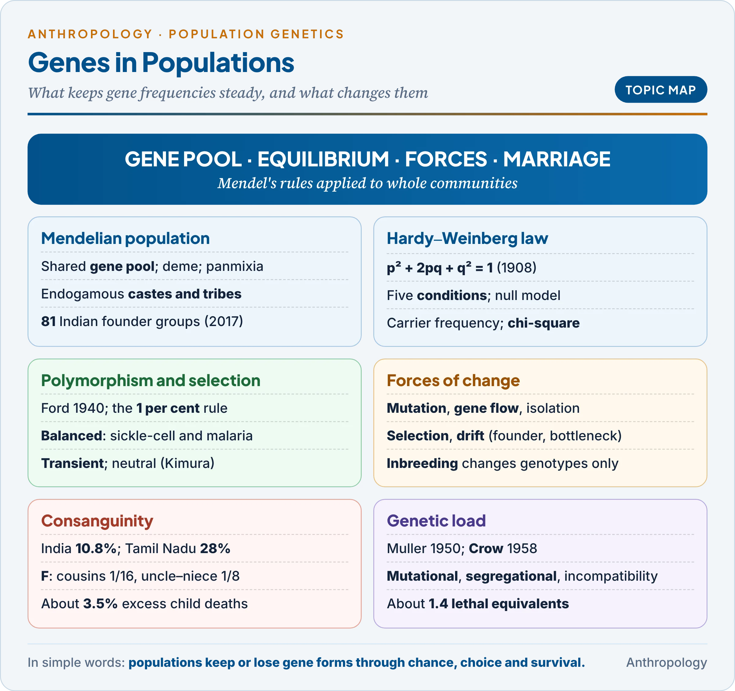
Unit 9.2 followed genes through families; this unit follows them through populations. A caste, a tribe or an island community can be treated as one pool of genes, and the question becomes: what keeps the proportions of alleles steady, and what changes them? The answer joins Mendel to Darwin. The forces of evolution were introduced in Unit 1.4b (in brief: mutation and gene flow bring in variation, drift and selection sort it, isolation lets populations diverge); here they are measured, applied to Indian populations, and linked to marriage rules.
1. Mendelian Population and Gene Pool
In simple words
A Mendelian population is a group of people who marry among themselves and so share one common stock of genes. Population genetics counts how often each form of a gene occurs in that stock. In India, an endogamous caste or tribe often behaves as such a population.
An example first. The Vysya, a trading community of Andhra Pradesh and Telangana of over 3 million people, have married within their community for centuries. A rare allele carried by a few early ancestors has therefore stayed inside the group and multiplied: the Vysya show about a 100-fold higher rate of butyrylcholinesterase deficiency (a dangerous reaction to certain anaesthetics) than other Indians (Nathan Nakatsuka and colleagues, 2017). The Vysya are a Mendelian population: their marriages define the boundary of a gene pool.
Definitions.
- Mendelian population: the term of the Russian-American geneticist Theodosius Dobzhansky: a reproductive community of sexual, cross-fertilising individuals who share a common gene pool. The largest Mendelian population is the species; the smallest is the local breeding unit.
- Deme: a local interbreeding population, the smallest Mendelian unit. A deme in which every individual is equally likely to mate with any other is panmictic (the American geneticist Sewall Wright‘s term panmixia).
- Gene pool: the sum of all alleles of all genes carried by the members of a population at one time. Each generation draws its genes from this pool, so the pool, not the individual, is what evolves.
- Allele frequency (gene frequency): the proportion of all copies of a gene in the pool that are of one type. Genotype frequency: the proportion of individuals with a given genotype.
Properties of a Mendelian population: continuity in time (the pool persists while individuals die), a boundary set by mating (in humans by culture as well as geography), and a measurable structure of allele and genotype frequencies.
The Indian application. Because caste and tribal endogamy restricts marriage, Indian groups living side by side can differ genetically.
- The Indian anthropologist Irawati Karve and K.C. Malhotra compared eight endogamous groups of the same rank in Maharashtra (Current Anthropology, 1968) and found significant differences between them, a pattern Malhotra later documented among the Dhangar (shepherd) castes.
- On a national scale, Nakatsuka and colleagues (Nature Genetics, 2017) studied over 2,800 people from over 260 South Asian groups and found 81 groups that descend from founder events stronger than those of Finns and Ashkenazi Jews; 14 of them number over a million people.
- Why it matters: each endogamous group can carry its own recessive diseases, which calls for community-specific carrier screening.
2. The Hardy–Weinberg Law
In simple words
The Hardy–Weinberg law says that if nothing disturbs a large, randomly mating population, the proportions of each gene form stay the same in every generation. It is the “no-change” baseline: when a real population departs from it, some force is at work.
2.1 Origin and statement
In 1908 the English mathematician G.H. Hardy (answering the geneticist R.C. Punnett) and the German physician Wilhelm Weinberg independently showed why a dominant allele does not automatically spread. The geneticist Curt Stern (1943) drew attention to Weinberg’s priority, and the rule came to be called the Hardy–Weinberg law.
Statement: in a large, randomly mating population, with no mutation, migration or selection, (1) allele frequencies remain constant from generation to generation, and (2) genotype frequencies reach p², 2pq and q² after one generation of random mating and stay there.
2.2 How it works
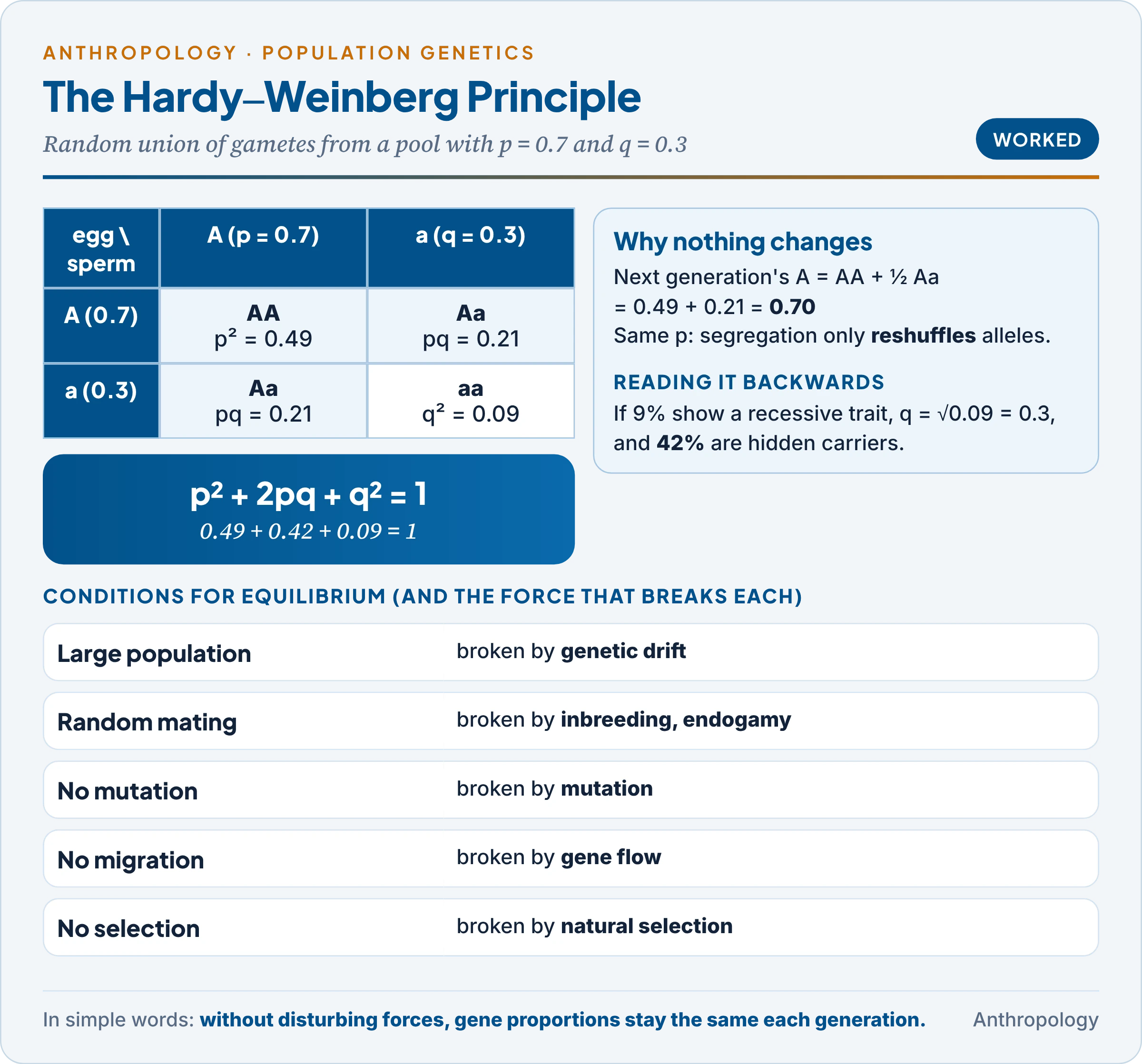
Let a gene have two alleles, A with frequency p and a with frequency q, so that p + q = 1.
- With random mating, every gamete is drawn at random from the pool: a sperm carries A with probability p and a with probability q, and so does an egg.
- The chance that a child gets A from both is p × p = p²; a from both, q²; one of each, pq + qp = 2pq.
- So (p + q)² = p² + 2pq + q² = 1.
- Why frequencies do not change: the next generation’s A alleles come from AA (all) and Aa (half), so the new p = p² + ½(2pq) = p(p + q) = p. Mendelian segregation only reshuffles alleles; it does not create or destroy them.
Extensions:
- Three alleles (ABO): with frequencies p (Iᴬ), q (Iᴮ) and r (i), (p + q + r)² = 1; group O = r², A = p² + 2pr, B = q² + 2qr, AB = 2pq (Worked Example 5).
- X-linked genes: in males the genotype frequency equals the allele frequency (q), in females it is q². If 8 per cent of men are colour-blind (q = 0.08), only about 0.64 per cent of women are, which matches observation.
2.3 Conditions for genetic equilibrium
The table lists the assumptions; the last column shows which evolutionary force breaks each one.
| Assumption | Why it is needed | Force that breaks it |
|---|---|---|
| Large population | Chance cannot change frequencies much | Genetic drift |
| Random mating (panmixia) | Gametes combine by chance | Inbreeding, assortative mating, endogamy |
| No mutation | No allele is converted into another | Mutation |
| No migration | No alleles enter or leave | Gene flow |
| No selection | All genotypes survive and reproduce equally | Natural selection |
| Sexual, diploid, non-overlapping generations | Simplifies the arithmetic | Real generations overlap (minor effect) |
The table shows why the law is the foundation of population genetics: each condition corresponds to one evolutionary force, so a population that departs from equilibrium tells us which force to look for. No real population meets all the conditions, yet most human populations come close for most genes, because the forces act slowly.
2.4 Importance and uses
- A null model: a population stays in equilibrium unless a force acts, so the law tells us when evolution (a change in allele frequency) has occurred.
- Estimating hidden carriers: from affected people (q²) we calculate carriers (2pq), whom the eye cannot see (Worked Example 2); this guides screening, as in India’s sickle-cell mission.
- Testing populations: observed counts are compared with expected ones by a chi-square test (Worked Examples 3 and 4); an excess of homozygotes points to inbreeding, endogamous subgroups or selection.
- Anthropology: allele frequencies of blood groups, haemoglobins or DNA markers measure genetic distance between castes and tribes.
- Why a dominant allele does not spread: dominance concerns how an allele shows, not how it is transmitted; without selection, a dominant allele at 10 per cent stays at 10 per cent, the point Hardy made in 1908.
3. Genetic Polymorphism and Selection
In simple words
A gene is polymorphic when two or more of its forms are each fairly common in a population, too common to be explained by fresh mutation alone. Something, usually natural selection, keeps them. Blood groups, haemoglobin types and the ability to taste PTC are familiar human examples.
An example first. In the Nilgiri Hills of Tamil Nadu in 1952, Hermann Lehmann and Marie Cutbush found the sickle-cell gene (HbS) among tribal people. It has since been found across central India, where the sickle-cell trait reaches 1 to 40 per cent of people in different tribal groups. HbS is harmful in double dose, yet it is common. Its frequency is too high to be renewed by mutation: it is kept by selection. This is the essence of genetic polymorphism.
3.1 Definition and levels
- Definition (the English geneticist E.B. Ford, 1940): “the occurrence together in the same locality of two or more discontinuous forms of a species in such proportions that the rarest of them cannot be maintained merely by recurrent mutation.”
- The 1 per cent rule of thumb: a locus is called polymorphic when its rarest common allele exceeds 1 per cent; rarer variants are attributed to mutation. A population with only one form is monomorphic.
- Polymorphic traits are discrete (taster or non-taster; group A or O) and largely genetic; continuous traits such as stature show variation, not polymorphism in Ford’s sense.
Levels at which polymorphism is found:
- Morphological (PTC tasting, ear-lobe attachment) and cellular: ABO, Rh, MN blood groups and HLA (human leucocyte antigens), the most polymorphic system known.
- Protein: haemoglobin variants (HbS, HbE, HbD), G6PD, haptoglobin. In 1966 Harry Harris (Britain) and Richard Lewontin and J.L. Hubby (USA) used electrophoresis (separating proteins in an electric field) to show that about a third of protein loci are polymorphic.
- Chromosomal: inversions and heteromorphisms visible under the microscope.
- DNA: single-nucleotide polymorphisms (SNPs), VNTRs (variable numbers of tandem repeats) and copy-number variants: the basis of DNA fingerprinting (Unit 9.1).
3.2 Types of polymorphism
Balanced polymorphism is kept stable by selection.
- Heterozygote advantage (overdominance): the heterozygote is fitter than both homozygotes, so both alleles are kept. Sickle-cell is the classic case (§3.3).
- Other malaria-linked cases: β-thalassaemia (proposed as malaria-protective by the British geneticist J.B.S. Haldane, 1949); HbE in north-east India; G6PD deficiency.
- Frequency-dependent selection (a form favoured while rare, as rare HLA types may resist local pathogens) and varying environments also keep polymorphisms stable. Sex itself is the most stable polymorphism: selection keeps the two sexes near 1 : 1.
- Disease and ABO: people of group O suffer more severe cholera, which may explain the low frequency of O in the cholera-endemic Ganges delta (Roger Glass and colleagues, 1985).
Transient polymorphism is a temporary stage while one allele replaces another under directional selection.
- Peppered moth (Biston betularia): dark forms rose in sooty industrial England (H.B.D. Kettlewell‘s experiments, 1950s) and fell again after clean-air laws.
- Lactase persistence (digesting milk sugar as adults) spread among dairying peoples over the last few thousand years.
Neutral polymorphism: the Japanese geneticist Motoo Kimura (1968) argued that most molecular variation is selectively neutral and changes by drift; many DNA polymorphisms are of this kind.
The table compares the three types; the last row gives the quickest way to tell them apart.
| Feature | Balanced | Transient | Neutral |
|---|---|---|---|
| Cause | Selection keeps both alleles | Selection replaces one allele | Drift; no selection |
| Duration | Stable, long-lasting | Temporary | Variable |
| Mechanism | Heterozygote advantage; frequency dependence | Directional selection | Random sampling |
| Examples | Sickle-cell, thalassaemia, HbE, G6PD | Peppered moth, lactase persistence | Most SNPs, many blood-group differences |
| Test | Frequencies steady over generations | Frequencies moving one way | Frequencies wander, linked to population size |
The table shows that the same visible pattern, two common forms, can arise from very different causes. Only long-term data or knowledge of fitness reveals which kind a polymorphism is.
Common confusion
Is a balanced polymorphism a sign that the harmful allele is “useful”? Only in a particular environment. HbS helps carriers where falciparum malaria is common; where malaria is controlled, the advantage vanishes and the allele slowly declines (relaxed selection). African Americans, removed from malaria for centuries, carry HbS at lower frequencies than West Africans, partly for this reason and partly through admixture.
3.3 Sickle-cell: a balanced polymorphism worked out
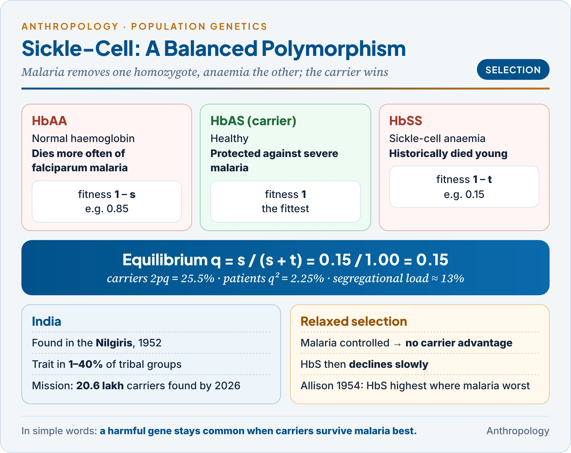
- The three genotypes:
- HbAA: normal haemoglobin but vulnerable to falciparum malaria.
- HbSS: sickle-cell anaemia, historically fatal in childhood without care.
- HbAS: sickle-cell trait, healthy and protected against severe malaria, because infected cells sickle and are removed by the spleen before the parasite multiplies.
- The proof: the British physician Anthony Allison (1954) showed in East Africa that HbS frequencies were highest where malaria was intense and that carriers had fewer parasites.
- The arithmetic: if the fitness of AA is reduced by s (malaria) and that of SS by t (anaemia), selection reaches equilibrium when q = s / (s + t). With s = 0.15 and t = 0.85, q = 0.15 and 25.5 per cent of people are carriers (Worked Example 8), close to the levels in parts of central India’s tribal belt.
- Natural selection on variation: this is how selection acts on genetic variety. It does not create alleles; it changes their frequencies through the differential reproduction of genotypes, measured by fitness (w) and the selection coefficient (s = 1 − w).
- Against a dominant harmful allele it is fast; against a rare recessive, very slow, because almost all copies hide in carriers (worked in Unit 1.4b).
- For heterozygotes it produces a stable equilibrium; against heterozygotes an unstable one, as in Rh incompatibility between mother and foetus.
- Other human cases: skin colour and ultraviolet light (Unit 9.2); the EPAS1 variant protecting Tibetans at altitude, inherited from Denisovans (Huerta-Sánchez and colleagues, 2014).
4. Forces That Change Gene Frequency
In simple words
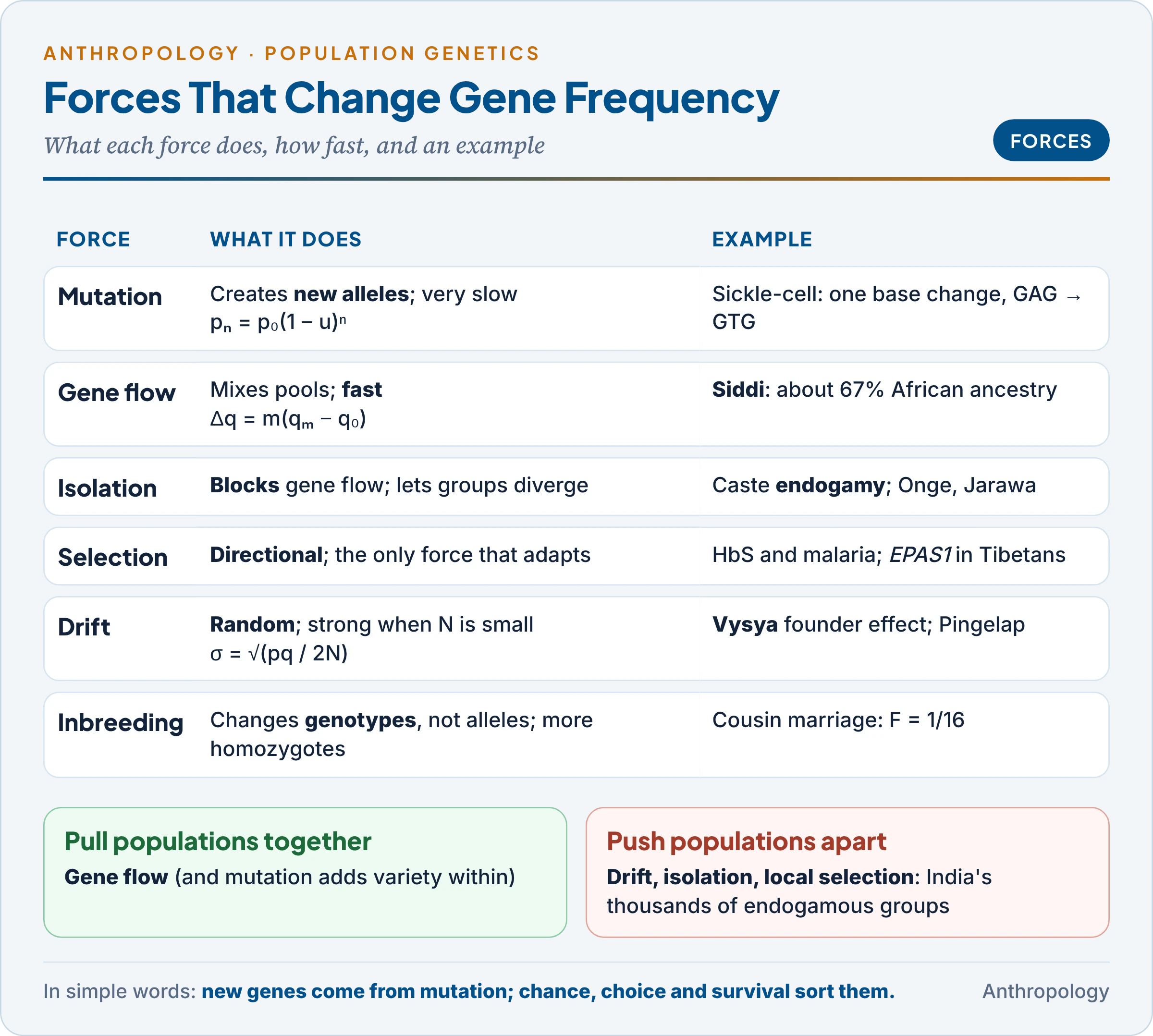
Six forces can push a population away from Hardy–Weinberg equilibrium: mutation, migration, isolation, selection, inbreeding and genetic drift. Some change how often an allele occurs; inbreeding changes only how alleles are paired. Together they explain why human populations differ.
4.1 Mutation
- What it is: a heritable change in DNA, the only source of new alleles (kinds in Unit 1.7).
- Mutation pressure: if A mutates to a at rate u per generation, after n generations pₙ = p₀(1 − u)ⁿ. Rates are about 1 in 100,000 to 1 in a million per gene, so p = 0.90 falls only to 0.891 in 1,000 generations (about 25,000 years) at u = 10⁻⁵.
- Two-way mutation: if a also mutates back to A at rate v, an equilibrium is reached at q = u / (u + v).
- Mutation–selection balance: a harmful recessive is removed by selection as fast as mutation creates it when q ≈ √(u/s), which explains why most disease alleles stay rare but never vanish.
4.2 Migration and gene flow
- What it is: movement of individuals and their genes between populations followed by interbreeding; called admixture or hybridisation when distinct populations merge.
- The formula: if a fraction m of a population’s parents are migrants with allele frequency qₘ, the new frequency is q₁ = (1 − m)q₀ + m qₘ, so the change is Δq = m(qₘ − q₀). Gene flow is fast compared with mutation: m = 0.2 can move q from 0.10 to 0.082 in one generation (Worked Example 7).
- Effects: gene flow makes populations more alike (reduces differences between them) and adds variety within each. It is the main counterweight to drift and isolation.
- Clines: gradual change in allele frequency across geography, such as the fall of blood group B from Central Asia westwards across Europe.
- Indian cases:
- The Siddi of Karnataka and Gujarat, descendants of Africans brought by the Portuguese, carry about 67 per cent African and 33 per cent Indian ancestry, from admixture about 8 generations (some 200 years) ago (Anish Shah and colleagues, 2011).
- Most Indian groups descend from mixture of Ancestral North Indians and Ancestral South Indians (David Reich and colleagues, 2009), followed by endogamy that froze the mixture about 2,000 years ago (Moorjani and colleagues, 2013).
4.3 Isolation
- What it is: any barrier that prevents gene flow: geographical (mountains, seas, forests), ecological, and in humans social and cultural (caste and tribal endogamy, religion, language).
- Effect: isolated populations diverge, because drift and local selection act on each separately; prolonged reproductive isolation in other species leads to speciation (isolating mechanisms in Unit 1.4b).
- Human isolates such as the Onge and Jarawa of the Andamans show low diversity; and Indian castes in one village behave as partly isolated gene pools, social distance replacing geographical distance.
4.4 Natural selection
Selection is the only force that adapts a population to its environment (forms and the sickle-cell case in §3). Its human agents are disease, climate and diet; modern medicine relaxes it.
4.5 Genetic drift
- What it is: random change in allele frequency due to chance in which individuals happen to reproduce; named the Sewall Wright effect after the geneticist who modelled it (1931).
- Size matters: the spread of chance change per generation is σ = √(pq / 2N). With p = q = 0.5, σ is 0.05 in a population of 50 but 0.005 in one of 5,000 (Worked Example 9). Drift is strong only in small populations.
- Outcomes: an allele is eventually lost or fixed, with a chance of fixation equal to its present frequency; drift reduces variation within populations and increases differences between them.
- Founder effect (the German-American biologist Ernst Mayr‘s “founder principle”, 1942): a new population started by a few founders carries only their alleles.
- The Old Order Amish of Lancaster County, Pennsylvania, have a high frequency of Ellis–van Creveld syndrome (dwarfism with extra fingers), traced to one founding couple (Victor McKusick, 1964).
- Tristan da Cunha in the South Atlantic, settled by a few families in the nineteenth century, has high retinitis pigmentosa and asthma.
- In India, the 81 founder groups of Nakatsuka and colleagues (§1) are the largest known set; the Vysya case shows the medical consequence.
- Bottleneck: a population shrinks sharply and recovers from a few survivors. A typhoon about 1775 left some 20 survivors on Pingelap atoll in Micronesia; today about 1 in 10 islanders has achromatopsia (total colour blindness). The Andamanese groups, reduced to a few hundred after colonial contact, show bottleneck effects.
4.6 Inbreeding and non-random mating
Inbreeding (mating of relatives) and assortative mating do not change allele frequencies; they change how alleles are combined, raising homozygotes at the expense of heterozygotes. Inbreeding thus exposes hidden recessives to selection, which can then change allele frequencies. It is treated in §5 and §6.
The table summarises how each force acts; notice that only mutation creates new alleles and only selection is directional.
| Force | Changes allele frequency? | Variation within a population | Differences between populations | Speed |
|---|---|---|---|---|
| Mutation | Yes, slightly | Increases | Increases | Very slow |
| Gene flow | Yes | Increases | Decreases | Fast |
| Isolation | Indirectly (lets others act) | — | Increases | Slow |
| Selection | Yes, directionally | Decreases (or keeps, if balancing) | Increases (different environments) | Depends on s |
| Drift | Yes, randomly | Decreases | Increases | Fast if N small |
| Inbreeding | No (genotypes only) | Fewer heterozygotes | Increases | Fast in close kin |
The table explains human diversity in one line: gene flow pulls populations together while drift, isolation and local selection push them apart, and the balance between these sets how different two populations become. India, with thousands of endogamous groups, is an extreme case of the “pushing apart” side.
5. Consanguineous and Non-consanguineous Mating
In simple words
Consanguineous marriage is marriage between relatives, such as cousins or an uncle and niece. Because relatives share genes from a common ancestor, their children are more likely to inherit two copies of the same harmful recessive gene. In South India such marriages are a long-standing preferred custom.
An example first. In much of Tamil Nadu and Karnataka, a man’s preferred bride has long been his mother’s brother’s daughter or, in some communities, his elder sister’s daughter. According to the National Family Health Survey 2019–21 (NFHS-5), about 28 per cent of marriages in Tamil Nadu and about 27 per cent in Karnataka were between blood relatives, against 10.8 per cent for India as a whole and only 4.4 per cent in Kerala (Tamil Nadu Economic Survey 2025–26). The same custom that builds alliances between families also concentrates genes.
5.1 Definitions
- Consanguineous mating: marriage between people who share at least one recent common ancestor; in clinical genetics, couples related as second cousins or closer (coefficient of inbreeding F ≥ 1/64 = 0.0156).
- Non-consanguineous mating: marriage between people not known to be related. It may be random (panmixia) or non-random:
- Positive assortative mating: like with like in phenotype: by stature, skin colour, education, or deafness among the deaf. It increases homozygosity for the genes behind the chosen trait only.
- Negative assortative (disassortative) mating: unlike with unlike; rare in humans as a conscious rule, though it may occur for some immune genes.
- Forms of consanguineous marriage in India (Unit 2.3 gives the social side: cross-cousin marriage builds alliances between descent groups, as in Dravidian kinship, while parallel-cousin marriage keeps property inside the lineage):
- Cross-cousin (MBD, FZD) and uncle–niece (elder sister’s daughter) marriage in the south; parallel-cousin (FBD) marriage among many Muslim communities.
- Incest (parent–child, brother–sister) is prohibited almost everywhere, though sibling marriage occurred in some royal lines (Egyptian pharaohs; Inca rulers).
The Indian pattern in numbers:
- NFHS-4 (2015–16): 9.9 per cent of marriages consanguineous; South 23 per cent, North-East 3.1 per cent; first cousins 8.7 per cent, second cousins 0.7, uncle–niece 0.6 per cent (Santosh Kumar Sharma and colleagues, 2020).
- Trend: prevalence fell from 14.4 per cent (1992–93) to 10.8 per cent (2019–21); 97 of 707 districts exceed 20 per cent, the top five in Karnataka and Tamil Nadu (Kumari and colleagues, 2026).
- Who: commoner among Muslims (about 16 per cent) than Hindus (about 10), and among the less educated and younger women, though in the south it cuts across class and caste. The Indian geneticist L.D. Sanghvi (1966) had documented high inbreeding in Andhra Pradesh.
- Reasons: keeping property in the family, lower dowry, security for the bride among known in-laws, and Dravidian kinship terms that mark cross cousins as marriageable.
Common confusion
Is inbreeding the same as consanguinity? Not exactly. Consanguinity is a social and genealogical fact: the couple are known relatives. Inbreeding is the genetic result: the chance that a child receives two copies of an ancestor’s allele. A small isolate or an endogamous caste can be inbred without any known consanguinity, simply because all its members descend from few founders.
6. Coefficient of Inbreeding and the Genetic Effects of Cousin Marriage
In simple words
The coefficient of inbreeding measures how closely the parents are related: the chance that their child gets two identical copies of a gene from one ancestor. For first cousins it is 1/16; for uncle and niece 1/8. The closer the relationship, the higher the risk of recessive disease.
6.1 The coefficient of inbreeding (F)
- Definition (Sewall Wright, 1922): F is the probability that the two alleles at a locus in an individual are identical by descent, that is, copies of the same ancestral allele.
- The path method: draw the path from the child’s father up to a common ancestor and down to the mother. If n is the number of people in the path (counting both parents and the ancestor), that ancestor contributes (½)ⁿ. Add the contributions of all common ancestors: F = Σ(½)ⁿ.
- First cousins: father → his parent → grandparent → her parent → mother = 5 people, so each grandparent gives (½)⁵ = 1/32; two shared grandparents give 1/16 = 0.0625.
- Uncle–niece: uncle → his parent → niece’s parent → niece = 4 people; (½)⁴ = 1/16 per ancestor; two ancestors give 1/8 = 0.125.
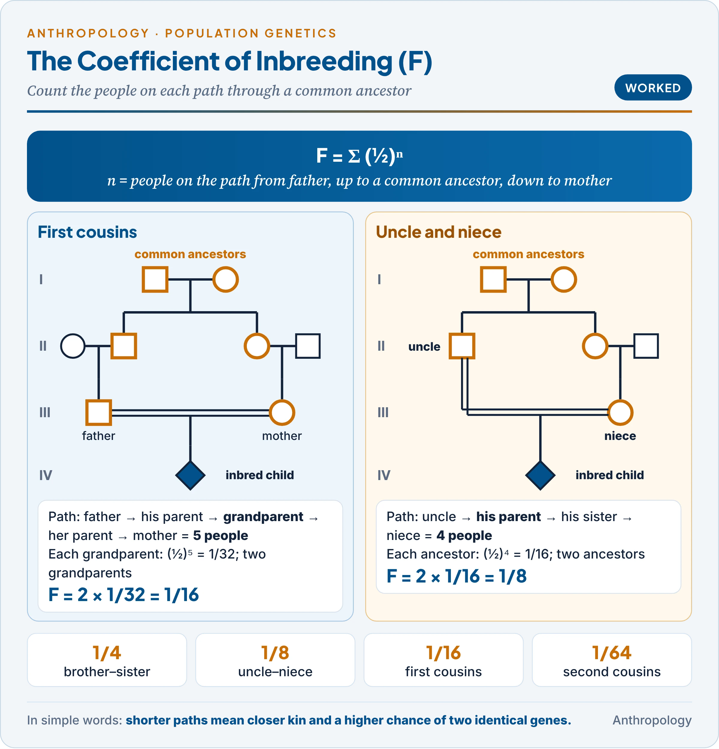
The table gives the values most often needed; note how each step away from close kinship halves or quarters the risk.
| Relationship of parents | F | As a decimal |
|---|---|---|
| Brother–sister; parent–child | 1/4 | 0.25 |
| Uncle–niece; double first cousins; half-siblings | 1/8 | 0.125 |
| First cousins | 1/16 | 0.0625 |
| First cousins once removed | 1/32 | 0.031 |
| Second cousins | 1/64 | 0.0156 |
| Unrelated (random mating) | 0 | 0 |
The table shows why uncle–niece marriage, common in parts of South India, carries twice the genetic risk of first-cousin marriage, and why second-cousin marriage adds very little.
6.2 What inbreeding does to genotypes
- With inbreeding, genotype frequencies become AA = p² + Fpq, Aa = 2pq(1 − F), aa = q² + Fpq. Heterozygotes fall by the fraction F; both homozygotes rise. Under the extreme of self-fertilisation in plants, heterozygosity halves every generation, from 0.5 to about 0.001 in ten generations.
- The risk of a recessive disease in a child of related parents is therefore q²(1 − F) + qF. The extra term qF is large compared with q² when q is small:
- For q = 0.01, first-cousin children are affected 7 times as often as children of unrelated parents; uncle–niece children 13 times.
- For q = 0.001, the ratios are 63 and 126 (Worked Example 10).
- Hence the rule: the rarer a recessive disease, the larger the share of cases from consanguineous marriages. Garrod noticed this for alkaptonuria in 1902.
6.3 The observed effects
- Mortality: a meta-analysis of 69 populations in 15 countries (2.14 million people) found about 3.5 per cent more deaths from late pregnancy to about 10 years among the children of first cousins than among children of unrelated parents (Alan Bittles and Michael Black, PNAS, 2010). An earlier estimate was 4.4 per cent (Bittles and James Neel, 1994).
- Morbidity and inbreeding depression: more autosomal recessive disorders (thalassaemia, spinal muscular atrophy, hearing and metabolic disorders), some malformations, and reduced growth or fitness in inbred offspring.
- Classic studies: William Schull and James Neel (The Effects of Inbreeding on Japanese Children, 1965) found small but real increases in mortality in Hiroshima and Nagasaki; in Karnataka, Bittles and Indian colleagues (Science, 1991) found raised stillbirth and infant death, though smaller than once feared.
6.4 “Inbreeding is not necessarily deleterious”
The statement, set by UPSC in 1981, holds in four senses:
- Inbreeding creates no harmful allele; it only reveals those already present. In a family with no deleterious recessives, cousin marriage carries no extra risk.
- The absolute extra risk is small: first-cousin children carry about 2–3 per cent additional risk of serious birth defects or early death, above a background of about 3 per cent for all births.
- Purging: where inbreeding has continued for many generations, harmful recessives exposed in homozygotes are removed by selection, so long-inbred populations may suffer less than expected.
- Social benefits (property, support, lower dowry) are real for the families concerned.
The opposite, outbreeding (crossbreeding or hybridisation), raises heterozygosity and can give hybrid vigour (heterosis) in crops and livestock; in humans it lowers recessive disease but confers no “superiority”.
7. Genetic Load
In simple words
Genetic load is the burden of harmful genes that every population carries. Because of it, the average person is a little less fit than the best possible genotype. Mutation, balanced polymorphism and inbreeding all add to the load.
Definitions. The American geneticist H.J. Muller introduced the idea in “Our Load of Mutations” (1950). James F. Crow (1958) defined genetic load as “the proportion by which the average fitness of a population is reduced in comparison with the best genotype“: L = (w_max − w̄) / w_max.
Types of genetic load:
- Mutational load: harmful alleles kept in the pool by recurrent mutation, balanced by selection. The Haldane–Muller principle states that each harmful mutation eventually causes one “genetic death” (failure to reproduce), whether mild or severe.
- Segregational (balanced) load: in a balanced polymorphism, the less fit homozygotes are produced in every generation by segregation. In the sickle-cell example, the population’s mean fitness is 0.8725 of the carriers’ fitness: a load of about 13 per cent (Worked Example 8).
- Incompatibility load: loss due to mother–foetus incompatibility, as in Rh haemolytic disease (erythroblastosis fetalis) when an Rh-negative mother carries an Rh-positive child.
How it is measured. Newton Morton, James Crow and H.J. Muller (1956) compared mortality in children of related and unrelated parents. The increase in death with F gives the number of lethal equivalents: sets of genes that, if all were homozygous, would cause one death. Human estimates are about 1.4 lethal equivalents per person acting between late pregnancy and age 10 (Bittles and Neel, 1994): each of us carries a few hidden recessive alleles that would be lethal in double dose.
Factors that influence genetic load:
- Mutation rate: raised by radiation, mutagenic chemicals and advanced paternal age.
- Inbreeding: exposes hidden load, converting it into deaths and disease.
- Medicine: relaxed selection lets carriers of once-lethal genes reproduce, so load accumulates slowly.
- Population size and environment: small groups fix harmful alleles by drift; an allele useful in one setting (HbS under malaria) becomes a load in another.
8. Worked Examples
In simple words
These examples show how allele, genotype and carrier frequencies are calculated, how equilibrium is tested, and how inbreeding raises risk. Each needs only simple arithmetic.
1. From non-tasters to all frequencies (PTC). In a sample, 30 per cent are non-tasters (tt).
- q² = 0.30, so q = √0.30 = 0.548 and p = 0.452.
- Homozygous tasters TT = p² = 0.205; heterozygous tasters Tt = 2pq = 0.495.
- Half of the population are hidden carriers of the non-taster allele.
2. Carrier frequency of a rare recessive. A disease affects 1 in 10,000 births.
- q² = 0.0001, so q = 0.01 and p = 0.99.
- Carriers 2pq = 2 × 0.99 × 0.01 = 0.0198, about 1 in 50 people.
- Lesson: carriers outnumber patients 200 to 1, and 99 per cent of the disease alleles sit in healthy carriers.
3. Testing equilibrium with chi-square (MN blood groups). Observed in 1,000 people: MM 298, MN 489, NN 213.
- Allele counting: p(M) = (2 × 298 + 489) / 2,000 = 0.5425; q(N) = 0.4575.
- Expected: MM = p² × 1,000 = 294.3; MN = 2pq × 1,000 = 496.4; NN = q² × 1,000 = 209.3.
- χ² = Σ (O − E)² / E = 0.046 + 0.110 + 0.065 = 0.22.
- Degrees of freedom = 3 classes − 1 − 1 (one allele frequency estimated) = 1; the critical value at P = 0.05 is 3.84.
- Since 0.22 < 3.84, the sample is in Hardy–Weinberg equilibrium.
4. A real departure (sickle-cell screening, Gadchiroli, Maharashtra). Under the national mission, 4,92,884 people were screened: 24,056 carriers (AS) and 2,654 patients (SS), so 4,66,174 were AA (Lok Sabha reply, 31 July 2026).
- q(S) = (2 × 2,654 + 24,056) / (2 × 4,92,884) = 0.0298.
- Expected SS = q² × N = 437; observed 2,654, about six times more. Expected AS = 28,489; observed 24,056, fewer.
- χ² is about 11,900 (1 d.f.): a massive excess of homozygotes. An inbreeding-type coefficient F = 1 − (observed AS / expected AS) = 1 − 24,056/28,489 ≈ 0.16.
- Why: (a) the district pools endogamous tribes with different frequencies (the Wahlund effect, after the Swedish geneticist Sten Wahlund, 1928: pooled groups always show fewer heterozygotes than expected); (b) consanguinity; (c) screening is not a random sample, since known patients come forward. The district is not one Mendelian population.
5. ABO with three alleles. Phenotypes: O 30, A 25, B 35, AB 10 per cent.
- r (i) = √0.30 = 0.548.
- p (Iᴬ) = 1 − √(B + O) = 1 − √0.65 = 0.194.
- q (Iᴮ) = 1 − √(A + O) = 1 − √0.55 = 0.258.
- Check: 0.548 + 0.194 + 0.258 ≈ 1.00. A high Iᴮ, as here, is typical of much of India.
6. Mutation pressure. p = 0.90, u = 10⁻⁵ per generation. After 1,000 generations, p = 0.90 × (1 − 10⁻⁵)¹⁰⁰⁰ = 0.891; with u = 10⁻⁶ it is still 0.899. Mutation alone changes populations almost imperceptibly.
7. Gene flow. A tribal village has HbS frequency q = 0.10. In one generation 20 per cent of parents come from a plains population with q = 0.01.
- q₁ = 0.8 × 0.10 + 0.2 × 0.01 = 0.082.
- One generation of gene flow outweighs thousands of generations of mutation.
8. Balanced polymorphism and segregational load. Fitness: AA = 1 − s = 0.85 (malaria), AS = 1, SS = 1 − t = 0.15 (anaemia).
- Equilibrium q = s / (s + t) = 0.15 / 1.00 = 0.15; carriers 2pq = 0.255; patients q² = 0.0225 (2.25 per cent of births).
- Mean fitness w̄ = 1 − s p² − t q² = 1 − 0.15 × 0.7225 − 0.85 × 0.0225 = 0.8725.
- Segregational load L = 1 − 0.8725 = 0.1275, about 13 per cent: the price of malaria protection.
9. Genetic drift and population size. With p = q = 0.5, σ = √(pq / 2N) is 0.05 for N = 50 (so 0.40–0.60 is common next generation), 0.016 for N = 500 and 0.005 for N = 5,000, where drift is almost negligible.
10. Risk from consanguinity. Risk of an affected child = q²(1 − F) + qF.
| Allele frequency (q) | Unrelated parents (F = 0) | First cousins (F = 1/16) | Uncle–niece (F = 1/8) |
|---|---|---|---|
| 0.01 | 1 in 10,000 | 7.2 in 10,000 (7 ×) | 13.4 in 10,000 (13 ×) |
| 0.001 | 1 in 1,000,000 | 63 in 1,000,000 (63 ×) | 126 in 1,000,000 (126 ×) |
The table shows the key consequence of cousin marriage: it raises the risk of rare recessive diseases far more, in relative terms, than of common ones.
Key Terms
| Term | Meaning in simple words |
|---|---|
| Mendelian population | A group that marries within itself and shares one gene pool |
| Gene pool | All the alleles carried by a population |
| Allele (gene) frequency | The share of all copies of a gene that are of one type |
| Hardy–Weinberg equilibrium | Unchanging allele and genotype frequencies without disturbing forces |
| Genetic polymorphism | Two or more common forms of a gene, the rarer above about 1 per cent |
| Balanced polymorphism | Two forms kept stable by selection, often because carriers are fitter |
| Transient polymorphism | Two forms present only while one is replacing the other |
| Genetic drift | Random change in allele frequency, strongest in small populations |
| Wahlund effect | Fewer heterozygotes than expected when separate groups are pooled |
| Consanguinity | Marriage between known blood relatives |
| Coefficient of inbreeding (F) | The chance that a child’s two alleles are copies of one ancestral allele |
| Genetic load | The reduction in average fitness caused by harmful genes |
| Lethal equivalent | A set of genes that would cause one death if all were homozygous |
Contemporary Developments
- Consanguinity mapped (August 2026): a district-level analysis of NFHS-5 found consanguinity fell from 14.4 per cent (1992–93) to 10.8 per cent (2019–21), with 97 of 707 districts above 20 per cent, the highest in Karnataka and Tamil Nadu (Kumari, Noolvi and Hallad).
- Sickle-cell screening (September 2026): over 7.3 crore people screened in tribal areas, with about 20.6 lakh carriers and 2.5 lakh patients identified; carriers receive cards and pre-marital counselling, a population-scale use of Hardy–Weinberg reasoning.
- GenomeIndia (April 2025): 9,772 genomes from 83 populations (30 tribal, 53 non-tribal) yielded about 180 million variants, most of them rare, supporting community-specific screening for founder diseases (Nature Genetics).
Diagrams to Master
- Topic map: Mendelian population → Hardy–Weinberg → polymorphism and selection → six forces → consanguinity and F → genetic load.
- Hardy–Weinberg square: gametes p and q on both sides; cells p², pq, pq, q²; write p² + 2pq + q² = 1 and the five conditions.
- Sickle-cell balance: three genotypes with fitness, malaria versus anaemia, q = s/(s + t).
- Forces: mutation, gene flow, isolation, selection, drift, inbreeding, each with its effect and one Indian example.
- Inbreeding paths: first-cousin pedigree with five-person paths through two grandparents (F = 1/16); uncle–niece with four-person paths (F = 1/8); mark the double marriage line.
Revision Grid
| Scholar | Work (year) | Key idea |
|---|---|---|
| Hardy; Weinberg | 1908 | Equilibrium of allele and genotype frequencies |
| Sewall Wright | 1922; 1931 | Coefficient of inbreeding; genetic drift |
| E.B. Ford | 1940 | Definition of genetic polymorphism |
| J.B.S. Haldane | 1949 | Malaria hypothesis for thalassaemia |
| H.J. Muller | “Our Load of Mutations” (1950) | Genetic load |
| Anthony Allison | 1954 | Sickle-cell trait protects against malaria |
| Morton, Crow and Muller | 1956 | Lethal equivalents |
| James F. Crow | 1958 | Formal definition of genetic load |
| Schull and Neel | The Effects of Inbreeding on Japanese Children (1965) | Effects of consanguinity |
| L.D. Sanghvi | 1966 | Inbreeding in India |
| Karve and Malhotra | 1968 | Genetic differences among endogamous groups |
| Motoo Kimura | 1968 | Neutral theory |
| Bittles and Black | PNAS (2010) | 3.5 per cent excess mortality in first-cousin offspring |
| Nakatsuka and colleagues | Nature Genetics (2017) | Strong founder events in 81 South Asian groups |
Previous Year Questions
Unit 9.3: Genetic polymorphism, Hardy–Weinberg law and consanguinity
- 2026Write notes on: Genetic polymorphism and natural selection.
- 2025What are genetic markers? Discuss their applications in understanding population variation, disease association and forensics.
- 2023What assumptions must be met for a population to be in genetic equilibrium? Explain the importance of genetic equilibrium.
- 2022Write notes on: Balanced and transient genetic polymorphism.
- 2022Discuss the role of evolutionary forces in creating human diversity.
- 2020Write notes on the Genetic drift in about 150 words.
- 2020How do marriage rules impact the gene pool of populations?
- 2019Differentiate between transient and balanced genetic polymorphism. Illustrate your answer with suitable examples from human populations.
- 2017Write a note in 150 words on Hardy-Weinberg Law.
- 2015Define genetic polymorphism. Give details of its types with suitable examples.
- 2015What do you understand by Immunogenetics? Explain with suitable examples.
- 2014Discuss the factors affecting gene frequencies among human populations.
- 2013What do you understand by ‘Genetic Load’ in a population? How is it measured and what are the important factors that can influence it? (250 words).
- 2012Write a note in 150 words on How ‘natural selection’ acts on variation?
- 2012What are the genetic effects of consanguinity? Give examples.
- 2011Write a note in 150 words on Conditions necessary for the operation of Hardy. Weinberg Law.
- 2011Write a note in 150 words on Genetic polymorphism.
- 2010What is Balanced Genetic Polymorphism? How is it maintained in a population?
- 2009Write a note on Natural selection in humans.
- 2009Write a note on Anthropological relevance of population genetics.
- 2009What is ‘genetic load’ & what factors influence it ?
- 2008Write a note on Inbreeding.
- 2008What do you understand by Hardy-Weinberg equilibrium? Discuss the factors that produce and redistribute variations.
- 2006Write a note on Genetic Polymorphism.
- 2005Write a note on Problems of Inbreeding.
- 2003Write a note on Genetic Polymorphism and Selection.
- 2003Describe in brief the major causes of change in gene frequency of a population.
- 2000Write a note on Genetic Adaptation.
- 1998Write a note on Mutation.
- 1998Define Hardy-Weinberg law and state briefly how Hardy-Weinberg law is applicable in population human genetics ?
- 1997Discuss the concept of ‘Mendelian population’ and its application in the study of anthropo-genetic variations in India.
- 1996Discuss the concepts of balanced polymorphism and relaxed selection with special reference to Malaria dependent polymorphisms in man.
- 1993Write a note on Inbreeding and crossbreeding.
- 1988Write a note on Inbreeding and hybridization.
- 1987Is inbreeding different from consanguinity? Give an account of inbreeding studies in India and comment on their social relevance.
- 1986What are the various forms of preferential mating? Explain with Indian examples.
- 1985Discuss the role of genetic drift, mutation and migration as the causes of variation.
- 1981‘Inbreeding is not necessarily deleterious in effect.’ Comment (200 words).
Related questions from other units
- 2026Unit 2.3: Discuss ‘incest taboo’ as the basis of development of kinship systems in human societies.
- 2024Unit 9.6: Write notes on: Hemoglobin in health and disease.
- 2021Unit 9.5: Write notes on : Is race a valid and biologically meaningful concept ?(in about 150 words).
- 2020Unit 1.4: Elucidate how Darwin and Post-Darwin theories of evolution resulted in the development of Synthetic theory of evolution.
- 2019Unit 1.7: Write a note in 150 words on Implications of mutation in evolution.
- 2018Unit 10: Explain the mechanisms of human variation in gene frequencies.
- 2015Unit 2.3: Write a note in 150 words on Incest Taboos.
- 2013Unit 9.6: What are genetic markers and what is their usefulness? Why are blood groups considered as good genetic markers? Illustrate with examples. (250 words).
- 1991Unit 10: Describe the stages of human physical growth and development and discuss the effect of nutrition and inbreeding on growth and development.
- 1988Unit 1.4: Give a critical account of the processes of organic evolution, and explain how they contribute to speciation.