- Species distributions have never been fixed: ice ages, mountain uplift and continental drift have reshuffled the biosphere many times. What marks the present episode is speed. Human-caused warming compresses change that once took millennia into decades, and many species cannot keep up with their shifting climate.
- A range shift is the movement of a species’ geographic distribution in response to changing conditions. It is a survival strategy: the species moves to stay inside a tolerable climatic envelope.
- A biogeographic response is the community-level outcome of many range shifts at once: altered species interactions, novel assemblages and restructured ecosystem functioning.
Range Shifts: Evidence and Mechanics

Why range shifts matter to biogeography
- Climate change is shifting species ranges in virtually every biome. It acts through rising temperature, changing precipitation and more frequent extremes (heatwaves, droughts, marine heatwaves), which together decide where suitable habitat lies.
- Because climate is the master control of distribution, range shifts are central to biodiversity conservation and ecosystem management, the applied wing of biogeography.
- Three consequences follow from a shifting climatic envelope:
- New species interactions arise as migrants meet species they have never shared a range with.
- Community composition changes, sometimes producing novel ecosystems with no analogue in the recent past.
- Conservation must become dynamic, moving from defending fixed areas to keeping connectivity, protecting climate refugia and even assisted migration.
Range shifts: a global phenomenon
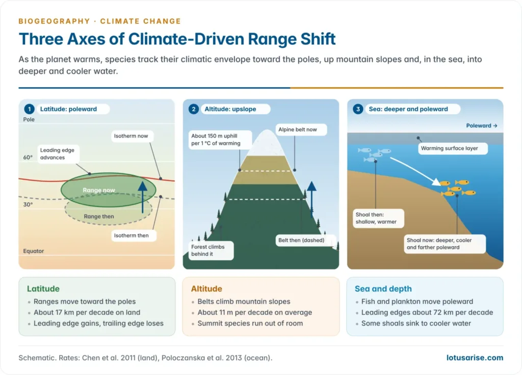
- A species can respond to warming in three ways: move, adapt in place or die out. Adapting in place needs rapid genetic or physiological change, so moving is the commonest response: the species tracks the location of its climatic niche across the landscape.
- Three well-documented kinds of shift are recognised: latitudinal, altitudinal and marine (including depth).
- The IPCC Sixth Assessment Report, Working Group II (2022), found that approximately half of the species assessed globally have shifted polewards or, on land, also to higher elevations (very high confidence).
Measured rates of shift
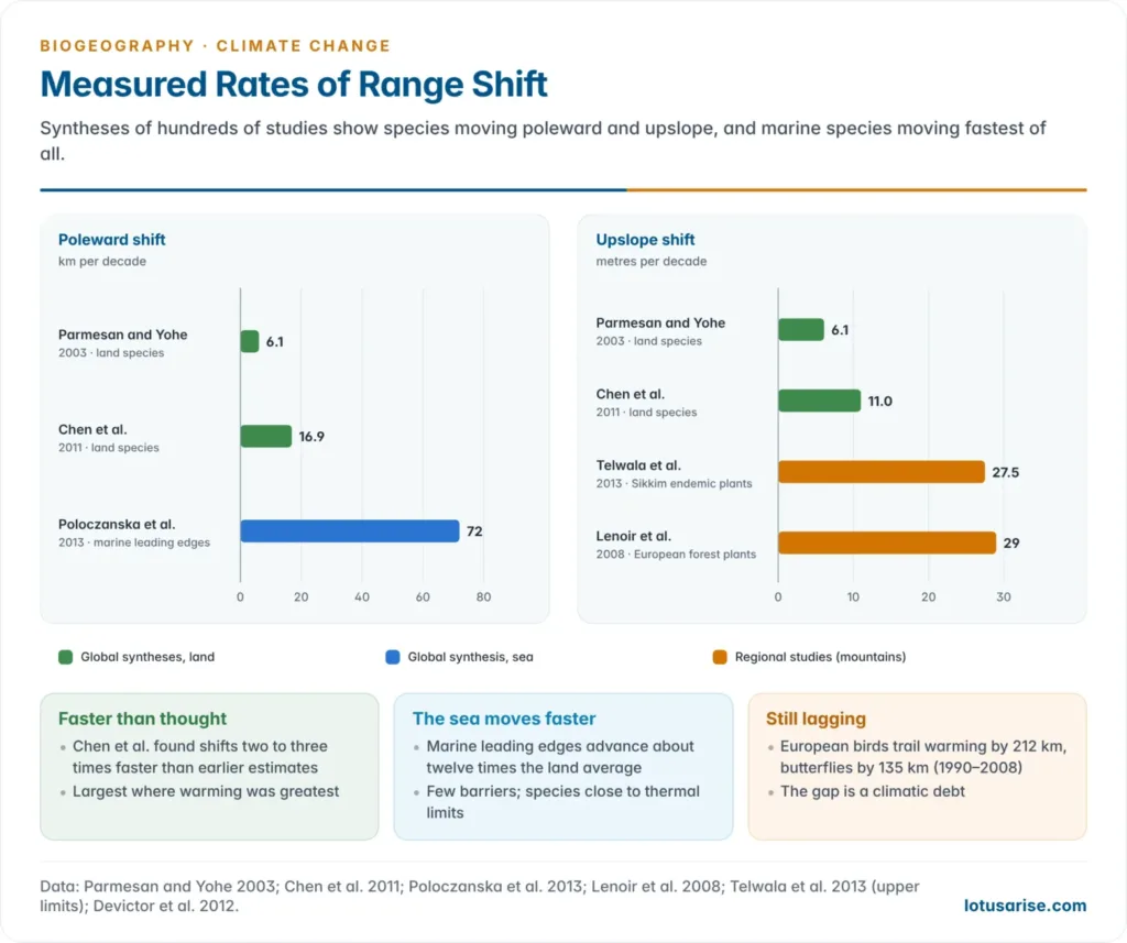
- Camille Parmesan and Gary Yohe (2003), analysing more than 1,700 species, found ranges moving about 6.1 km per decade poleward (or 6.1 m per decade upslope).
- I-Ching Chen, Chris Thomas and colleagues (2011) found median shifts of 16.9 km per decade to higher latitudes and 11.0 m per decade to higher elevations: two to three times faster than earlier estimates. The largest shifts occurred where warming was greatest, a direct fingerprint of climate.
- A global synthesis of 30,534 range shifts in over 12,000 species (Jonathan Lenoir and colleagues, 2020) found marine species moving poleward up to six times faster than terrestrial ones.
| Study | Group | Rate of shift |
|---|---|---|
| Parmesan and Yohe (2003) | Mostly land, Northern Hemisphere | 6.1 km per decade poleward; 6.1 m per decade upslope |
| Chen et al. (2011) | Land | 16.9 km per decade poleward; 11.0 m per decade upslope |
| Lenoir et al. (2008) | Forest plants, western Europe | Optimum elevation up 29 m per decade |
| Poloczanska et al. (2013) | Ocean (plankton, fish) | Leading edges 72 km per decade poleward |
| Dulvy et al. (2008) | North Sea bottom fish | 3.6 m per decade deeper |
Latitudinal range shifts
- The best-documented shift is poleward: northward in the Northern Hemisphere, southward in the Southern. Cool-adapted species follow the retreat of their thermal zone toward higher latitudes.
- Alan Hitch and Paul Leberg (2007) found that the northern range limits of 56 North American bird species moved north over 26 years, while their southern limits stayed put.
- Leading edges usually advance faster than trailing edges retreat, so many ranges first widen and then shift.
- Shifts are not uniform. Birds and butterflies, which disperse easily, track climate more readily than slow-dispersing plants or habitat specialists.
- Even mobile groups lag. Across Europe (1990–2008), bird communities trailed the northward shift of temperature by 212 km and butterflies by 135 km (Vincent Devictor and colleagues, 2012). This climatic debt leaves communities out of step with their climate.
Altitudinal range shifts
- In mountains, species escape warming lowlands by moving upslope: the montane analogue of a poleward shift, packed into a short distance.
- Temperature falls about 6.5 °C per 1,000 m (the environmental lapse rate), so 1 °C of warming lifts a thermal zone about 150 m.
- Examples:
- The optimum elevation of 171 forest plants in western Europe rose about 29 m per decade (1905–1985 to 1986–2005) (Jonathan Lenoir and colleagues, 2008).
- Moths on Mount Kinabalu, Borneo, moved uphill an average of 67 m in 42 years (1965–2007).
- The squeeze at the top: as zones climb, mountaintop species lose area and finally run out of mountain, the “escalator to extinction”. Such range contractions and local extinctions are the end point of upslope shifts.
- Not every shift is upward. Many Californian plants moved their optimum elevation downhill by about 80 m (1930s to 2000s), because higher rainfall improved the water balance of lower slopes (Shawn Crimmins and colleagues, 2011). Species track the whole climatic niche, not temperature alone.
The Himalaya: treelines and upslope shifts
- The Hindu Kush Himalaya warmed by about 1.3 °C between 1951 and 2014 (Ministry of Earth Sciences, 2020).
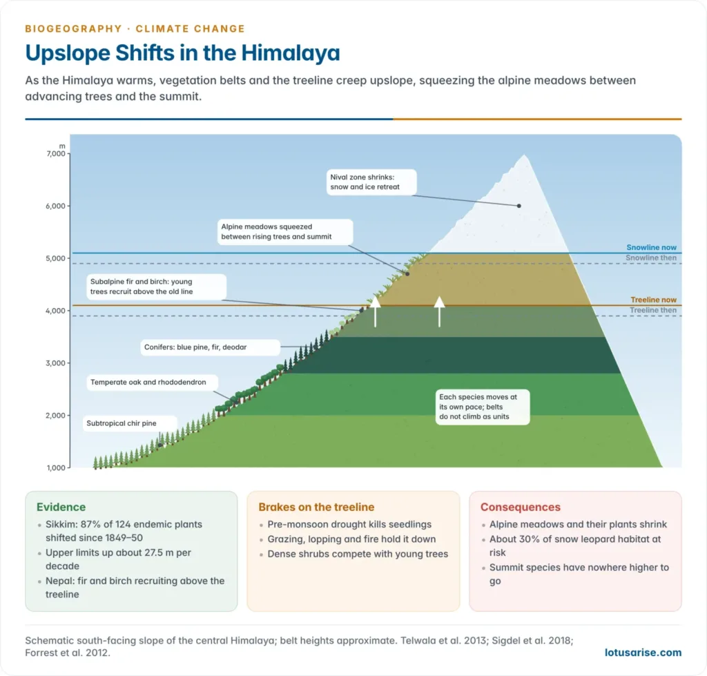
- Sikkim Himalaya: Yasmeen Telwala and colleagues (2013) compared 124 endemic plants with the records Joseph Dalton Hooker made in 1849–50.
- 87% had shifted, mostly upslope. Upper limits rose 23 to 998 m, an average of about 27.5 m per decade.
- Species richness has risen in the upper alpine zone as lower species climbed into it.
- Treelines: a 2023 satellite study of 243 mountain regions found 70% of treelines moved upslope between 2000 and 2010, about 1.2 m a year on average. Himalayan treelines respond more slowly and unevenly:
- Moisture matters as much as temperature. Treelines advance where spring is wet enough for seedlings and lag where pre-monsoon drought kills them (Shalik Ram Sigdel and colleagues, 2018).
- In Nepal, Abies spectabilis (Himalayan fir) and Betula utilis (Himalayan birch) treelines show consistent upward recruitment.
- Many Himalayan treelines are held down by grazing, lopping and fire, or are dwarf krummholz belts. They respond first by densification, not by advance.
- Species interactions slow the climb: on the Tibetan Plateau, dense shrub belts kept fir treelines stable for a century, while sites with sparse shrubs advanced up to 80 m (Eryuan Liang and colleagues, 2016).
- Consequences: a rising treeline shrinks alpine meadows. About 30% of the snow leopard’s Himalayan habitat could be lost to treeline shift under continued high emissions (WWF study, 2012). The belts of the mountain biome climb together, but not in step.
Marine range shifts
- Ocean warming drives comparable shifts: fish, plankton and invertebrates move toward the poles or into deeper, cooler water.
- North Sea: Allison Perry and colleagues (2005) found that nearly two-thirds of 36 bottom-living fish species shifted their mean latitude, depth or both over 25 years, as bottom water warmed by about 1 °C.
- Half the species with range edges in the North Sea shifted their boundaries, nearly all northward. Smaller, faster-maturing species moved most.
- The fish assemblage deepened about 3.6 m per decade (1980–2004).
- Globally, marine leading edges have advanced about 72 km per decade (Elvira Poloczanska and colleagues, 2013), about twelve times the land average of about 6 km per decade.
- Why the sea moves faster: fewer barriers, larvae drifting on currents, and cold-blooded species living close to their thermal limits, with no shade or altitude to retreat into.
- Marine taxa follow their local isotherms, which may run east, west or even south (Malin Pinsky and colleagues, 2013).
- Indian seas:
- The oil sardine, once confined to the Malabar upwelling zone (8°N–14°N), has extended north of 14°N: by 2006 that coast gave about 15% of India’s catch. It has also spread into the Bay of Bengal.
- The Indian mackerel is moving deeper: bottom trawlers took about 2% of its catch in 1985–89 and about 15% in 2003–07.
- Both track rising sea surface temperature.
The velocity of climate change
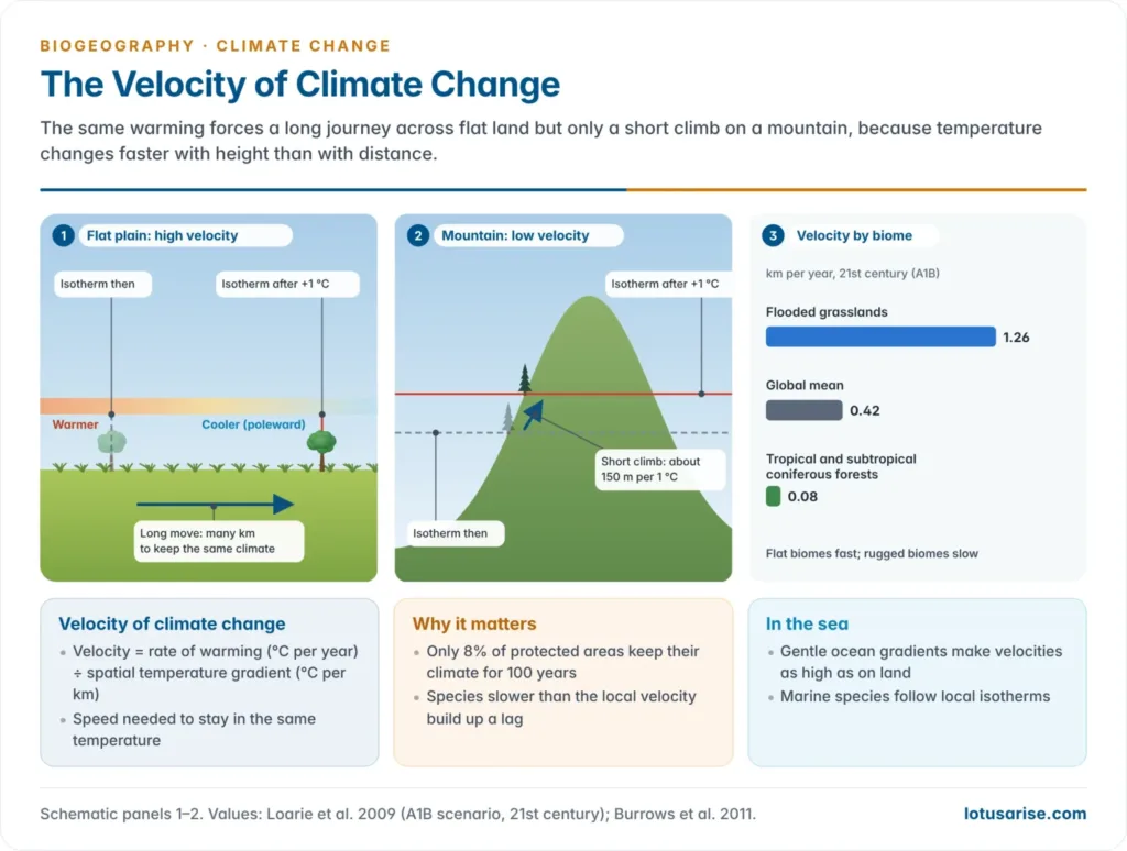
- The velocity of climate change (Scott Loarie and colleagues, 2009) is the speed at which a species must move across the surface to stay in the same temperature.
- Velocity (km per year) = rate of warming (°C per year) ÷ spatial temperature gradient (°C per km).
- Where temperature changes sharply over short distances (mountains), velocity is low; on flat land a species must travel far.
- Findings (21st century, A1B emissions scenario):
- Global mean: about 0.42 km per year.
- Lowest in rugged biomes, such as tropical and subtropical coniferous forests (about 0.08 km per year).
- Highest in flat biomes: flooded grasslands (1.26 km per year), mangroves and deserts.
- Only 8% of protected areas have climates that will persist inside their boundaries for more than 100 years.
- Mountains are climate shelters; plains, deltas and coastal flats are where species are most likely to be left behind.
- Ocean temperature gradients are gentle, so despite slower warming, ocean velocities are as high as those on land (Michael Burrows and colleagues, 2011).
- Where a species’ dispersal speed is lower than the local velocity, it builds up a lag. Many trees, spreading seed tens of metres a year, cannot keep pace on lowland plains.
Biogeographic Responses Beyond the Individual Species
- Range shifts cascade into community-level and ecosystem-level responses: changed species interactions, changed community composition and a new conservation problem.
Changes in species interactions
- Migrants meet organisms with which they share no evolutionary history of competition, predation or mutualism. These novel interactions can ripple through an ecosystem with disproportionate effect.
- A migrant may replace the residents, fail and die out, coexist with them, colonise vacant niches or interbreed to form hybrids.
- Examples:
- Red fox and Arctic fox: the larger red fox is spreading north into tundra and displacing the Arctic fox from dens and food.
- A wild grizzly–polar bear hybrid was confirmed by DNA in the Canadian Arctic in 2006.
- Milder winters let the mountain pine beetle cross the Rockies into Alberta’s pine forests, reaching hosts it had not met before.
- Tropical rabbitfish moving poleward have overgrazed kelp forests off Japan and Australia, a process called tropicalisation.
- Timing mismatches add to spatial ones when predators and prey, or flowers and pollinators, fall out of phenological step.
Changes in community composition: novel communities
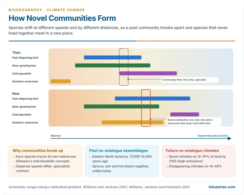
- Species shift at different rates and in different directions, so the mix at any place changes. This produces novel communities: assemblages of species that have not co-occurred before, with unpredictable consequences for ecosystem functioning.
- Communities do not move as units because each species responds to its own tolerances, as Henry Allan Gleason (1926) argued in his individualistic concept. Communities disassemble and reassemble.
- No-analogue assemblages of the past: in eastern North America, 17,000–12,000 years ago, spruce, ash, hornbeam and other trees grew together in combinations not found anywhere today, under climates that no longer exist (John Williams and Stephen Jackson, 2007).
- Such late Pleistocene assemblages show that novel communities are a normal outcome of rapid climate change.
- No-analogue climates of the future: under high emissions, by 2100,
- novel climates could cover 12–39% of the land, mostly in the tropics and subtropics;
- disappearing climates could cover 10–48%, especially tropical mountains and the poleward edges of continents;
- under low emissions, both shrink to 4–20%.
- Novel ecosystems (Richard Hobbs and colleagues, 2006) have been changed irreversibly by climate, invasions and land use. Restoring a historical baseline is often impossible, so management aims at function and resilience.
Conservation Challenges and the Problem of Prediction
Conservation challenges posed by dynamic ranges
- Traditional conservation assumed static protected areas: draw a boundary around a habitat and defend it. Range shifts undermine this premise in two ways.
The connectivity problem
- Species must move physically to track their climate. Fragmented landscapes and barriers (roads, farmland, urban sprawl) block them from newly suitable habitat even where it exists.
- With only 8% of protected areas likely to keep their climate for a century, reserves become way stations rather than permanent homes. Habitat fragmentation turns climate change into an extinction threat.
The predictive uncertainty problem
- Climate models give general projections of temperature and precipitation. Far less certain is how any particular species will respond, especially once novel interactions are added.
- Why range shifts are hard to predict:
- Species distribution models assume equilibrium: a species fills all the climate it tolerates and keeps the same niche. Lagging species break both assumptions.
- Dispersal limits and barriers are often left out.
- Biotic interactions, evolution and plasticity can widen or narrow the real range.
- Climate dimensions conflict: warming pushes species uphill, water balance can pull them down.
- Microclimates (shaded gullies, cold-air pools) shelter populations that coarse grids miss.
- No-analogue climates lie outside the conditions models were trained on.
- Evidence is biased toward Europe and North America; the tropics and South Asia are poorly sampled.
- Projections are therefore scenarios with uncertainty, and planners prefer strategies that work under many futures.
Adaptive conservation strategies
- Conservation now treats distributions as moving targets, not fixed points. The strategies for conservation under climate change fall into three groups:
| Strategy | Mechanism | Illustrative example |
|---|---|---|
| Ecological corridors | Connected habitat linkages so species can move between fragmented patches | Yellowstone to Yukon Conservation Initiative, a continental-scale connected landscape (Hilty et al., 2020); Terai Arc Landscape, India and Nepal |
| Climate refugia | Protecting areas expected to stay climatically stable despite wider warming | Cool, moist microhabitats in mountains; deep valleys of the Eastern Himalaya |
| Assisted migration | Deliberate human relocation of species to places expected to become suitable | Controversial: risks introducing invasive species or disrupting the recipient ecosystem |
Previous Year Questions
- No direct PYQ has been asked on this sub-topic yet.