The t-test and Two-Way ANOVA: Assumptions, Worked Example and Interaction

Application of statistical technique (t-test, two way ANOVA).

Official Syllabus: Paper I · Unit 3 Research Methods

“The null hypothesis is never proved or established, but is possibly disproved, in the course of experimentation.”

— Fisher (1935)

A statistical test does not tell the investigator whether a hypothesis is true. It reports how improbable the obtained data would be if nothing were going on, and the apparatus below is built on that asymmetry. Which test applies is settled before the data arrive, by three things only: the scale on which the dependent variable is measured, the number and relatedness of the groups compared, and the assumptions the data can be expected to meet.

Scales of measurement and what they permit

Stevens (1946) classified measurement into four scales, and the classification matters because it determines which arithmetic is meaningful.

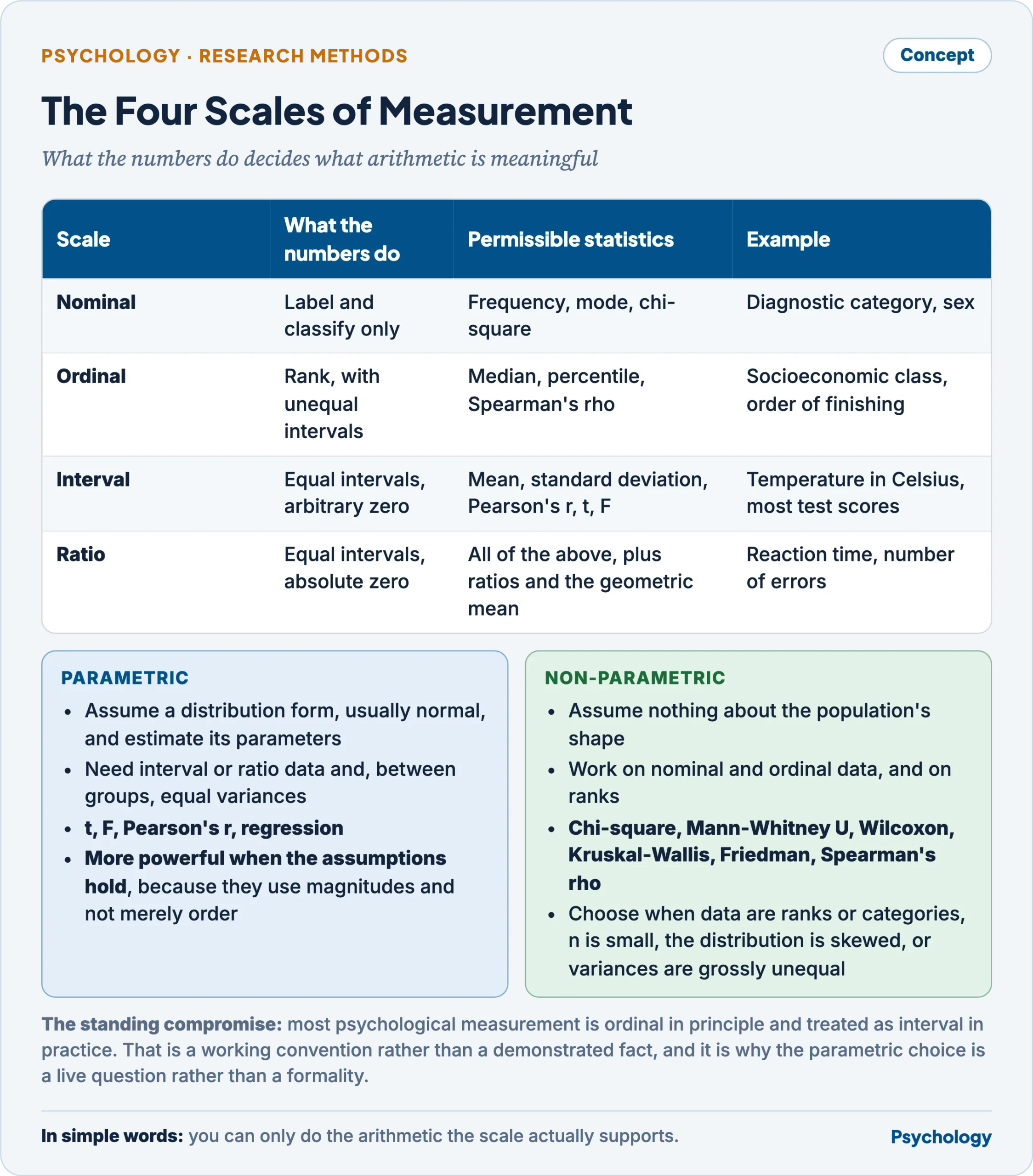
The scale decides which arithmetic is meaningful, and so which test applies.

Most psychological measurement is ordinal in principle and treated as interval in practice. That is a working compromise rather than a demonstrated fact, and it is the reason the parametric choice below is a live question rather than a formality.

Parametric and non-parametric statistics

• Parametric tests assume that the population sampled has a specified distribution form, usually normal, and they estimate its parameters. They require interval or ratio data and, for between-group tests, homogeneity of variance. The t-test, ANOVA, Pearson’s correlation and regression are all parametric.
• Non-parametric tests, also called distribution-free, make no assumption about the population’s shape. They work on nominal or ordinal data and on ranks derived from interval data. Chi-square, the Mann-Whitney U test, the Wilcoxon signed-rank test, the Kruskal-Wallis test, Friedman’s test and Spearman’s rho are the standard set.
• The trade. When their assumptions hold, parametric tests are more powerful, because they use the magnitudes in the data and not merely the order. When the assumptions fail, the parametric test’s stated error rate is no longer its real one, and the non-parametric test becomes the honest choice. The loss in power is smaller than usually supposed: under normality the Mann-Whitney U is only slightly less efficient than the t-test, and where the distribution is skewed it can be the more powerful of the two.
• When to prefer a non-parametric procedure — the dependent variable is a rank or a category; the sample is too small for normality to be assessed; the distribution is markedly skewed or carries extreme outliers; variances are grossly unequal; or scores are censored at a ceiling or floor.
• Matching the problem to the test. Whether a new syllabus raises examination marks is a parametric problem — interval scores, two groups, a t-test. Whether candidates prefer one of three selection procedures is non-parametric — a nominal outcome, tested by chi-square. Whether the rank order of job applicants given by two interviewers agrees is Spearman’s rho. Whether severity ratings on a four-point clinical scale improve after therapy is Wilcoxon’s signed-rank test.

The t-test

Student (1908) — the pseudonym of W. S. Gosset, working on small samples at a brewery — derived the distribution that makes inference possible when the population standard deviation is unknown and must be estimated from the sample. The t distribution is flatter and wider in the tails than the normal, and approaches it as degrees of freedom grow.

The three basic conditions for its use

• The dependent variable is measured on an interval or ratio scale, so that means and standard deviations are meaningful quantities.
• The populations sampled are normally distributed on that variable. With samples above about thirty the central limit theorem makes the test robust to moderate departures.
• Homogeneity of variance — the two populations compared have equal variances — together with independence of observations within each group. Where variances differ sharply and group sizes are unequal, Welch’s correction replaces the pooled estimate.

A fourth constraint follows from the test’s structure rather than its assumptions: it compares not more than two means at a time.

Five uses

• One-sample t-test — a sample mean against a known or hypothesised population value, as when a school’s mean score is tested against the published test norm.
• Independent-samples t-test — the means of two unrelated groups, as when an experimental and a control group are compared after training.
• Paired-samples t-test, also called correlated or dependent samples — two related means, from the same people measured twice or from matched pairs. Because each person serves as their own control, it is markedly more powerful than the independent-samples form on the same number of observations.
• Testing the significance of a correlation coefficient, through the identity t = r × √(n − 2) ÷ √(1 − r²), evaluated at n − 2 degrees of freedom.
• Testing the significance of a regression coefficient, where t is the coefficient divided by its standard error. This is how each predictor in a regression is judged, and it is also how the difference between two proportions is tested in large samples.

A worked independent-samples t-test

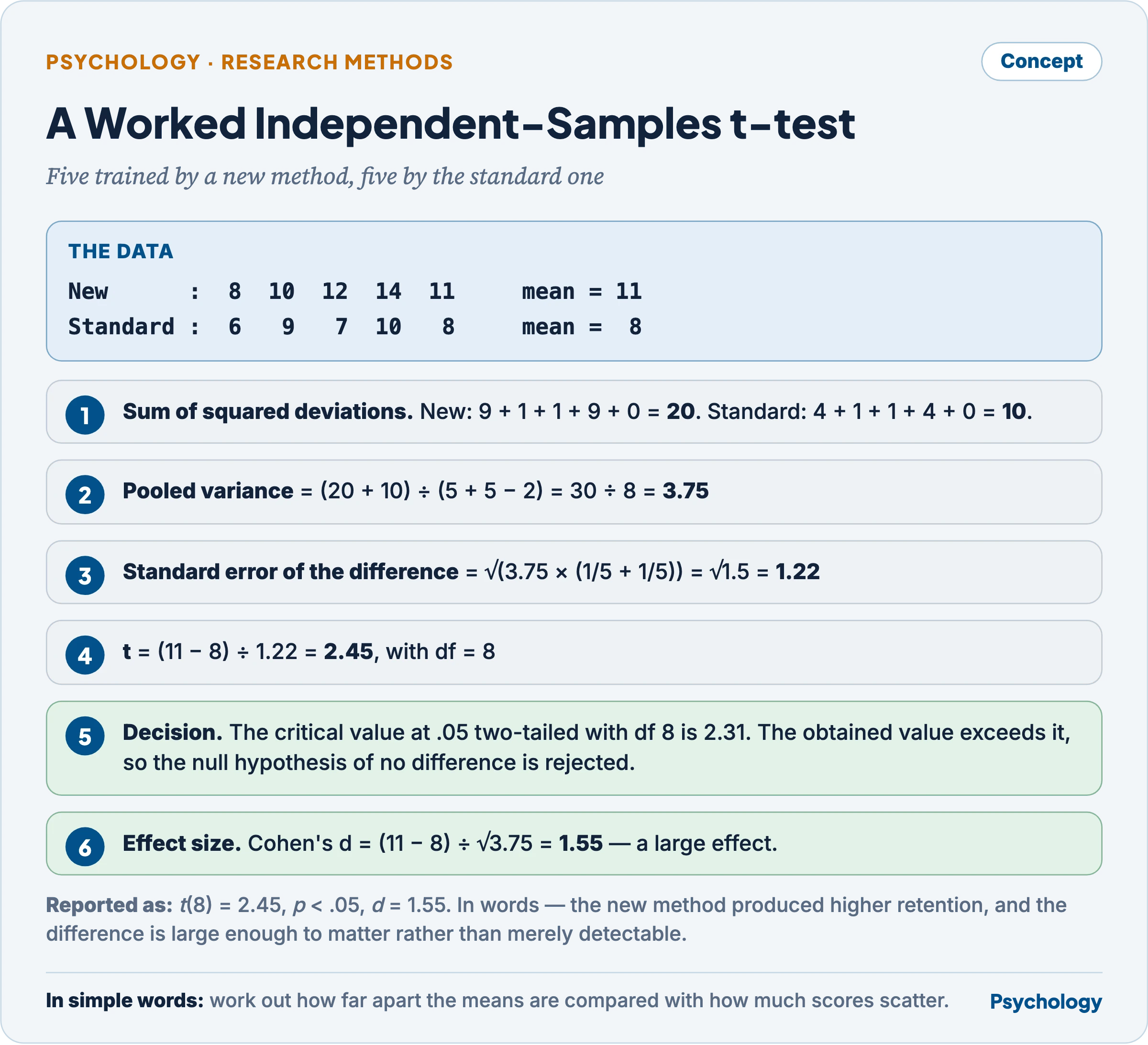
Five trained by a new method, five by the standard one.

Reported as: t(8) = 2.45, p < .05, d = 1.55. In words, the new method produced higher retention, and the difference is large enough to matter rather than merely detectable.

What happens when the assumptions fail

Non-normality with equal and reasonably large groups leaves the test’s error rate near its stated level. Unequal variances combined with unequal group sizes is the dangerous case: the real error rate departs from the nominal one in a direction that depends on which group is larger, and Welch’s test is the remedy. Non-independence of observations — repeated measures analysed as independent, or participants nested within classrooms — inflates the Type I error rate severely and has no correction inside the t-test; it requires a different model altogether.

Analysis of variance

Why not repeated t-tests

With three groups there are three pairwise comparisons, with four groups six. Each test carried out at the .05 level carries its own chance of a false positive, so the probability that at least one comparison is spuriously significant rises with their number — about .14 for three comparisons and about .26 for six. Analysis of variance tests the whole set of means in one procedure at one stated error rate, and that is its reason for existing.

Partitioning variance

The logic is a partition. The total variability of all scores about the grand mean is divided into variability between groups, which carries treatment effect plus error, and variability within groups, which carries error alone. Each sum of squares is divided by its degrees of freedom to give a mean square, and

F = MS between  /  MS within
    df = (k - 1)  and  (N - k)

If the treatments do nothing, both mean squares estimate the same error variance and F is near 1. An F substantially greater than 1 is evidence that the between-groups term contains something beyond error. A significant F with more than two groups says only that the means are not all equal; post hoc comparisons such as Tukey’s test identify which pairs differ.

Assumptions of ANOVA

• Independence of observations — each score is unaffected by every other, which follows from random sampling and random assignment.
• Normality — the dependent variable is normally distributed in each population sampled.
• Homogeneity of variance — the scatter of scores is the same across all groups. Levene’s test is the usual check, and Welch’s or Brown-Forsythe’s F the usual remedy.
• Interval or ratio measurement of the dependent variable, and additivity of the effects in the underlying model.

On violation: F is robust to non-normality when group sizes are equal and moderate. It is robust to heterogeneity of variance only when group sizes are equal; with unequal sizes the error rate is distorted, and badly so when the larger group has the smaller variance. Violation of independence is the one failure with no repair inside the model.

Two-way ANOVA

A two-way ANOVA has two independent variables, called factors, each with two or more levels, crossed so that every combination is represented. It partitions the between-groups variability three ways and tests three null hypotheses at once:

• the main effect of A — the effect of the first factor, averaged across the levels of the second;
• the main effect of B — the effect of the second factor, averaged across the levels of the first;
• the A × B interaction — whether the effect of one factor depends on the level of the other.

SS total = SS A + SS B + SS AB + SS within

Its assumptions are those of one-way ANOVA, with one addition that the crossed structure creates: the design should be balanced, or near enough, since with markedly unequal cell sizes the sums of squares are no longer independent and the order in which effects are entered changes the result.

It is not two one-way ANOVAs added together

This is the heart of the technique and the reason the design exists, and it rests on four distinct points.

• The interaction is new information that no one-way analysis can yield. Two separate one-way analyses produce the two main effects and nothing else. The interaction term exists only because the factors were crossed in one design, and it is frequently the finding that matters — a teaching method that helps anxious learners and hinders calm ones.
• The error term is smaller, so every test is more powerful. In a one-way analysis of factor A alone, all the variability produced by factor B falls into the within-groups error term. In the two-way design that variability is extracted as the sum of squares for B, leaving a smaller mean square within. The same data therefore give a more sensitive test of A.
• A main effect can be uninterpretable on its own. When the interaction is significant, a main effect is an average across conditions in which the factor acted in opposite directions, and it may describe nobody in the study. The correct follow-up is an analysis of simple effects — the effect of A at each level of B separately — not a reading of the main effect.
• Economy and generality. One set of participants tests two hypotheses with fewer people than two separate studies would need, and each main effect is established across the levels of the other factor rather than at one arbitrary setting of it, so it generalises further.

Merits, applications and interpretation

The merits follow directly: a simultaneous test of two factors and their joint action at one controlled error rate; detection of moderation, which is what an interaction is; reduced error variance and so greater power; efficient use of participants; and broader generalisability of each main effect.

In psychological research it is applied wherever a second variable is expected to qualify the first — drug type crossed with dosage on anxiety reduction; teaching method crossed with learner anxiety on achievement; sex crossed with length of a training programme on performance; stimulus modality crossed with retention interval on recall.

A hypothetical interpretation. Suppose sex, at two levels, is crossed with the duration of an exercise programme, at three levels, on a fitness score, with eight participants per cell. The analysis returns a significant main effect of sex, F(1, 42) = 22.37, p < .001; a significant main effect of programme duration, F(2, 42) = 36.03, p < .001; and a non-significant interaction, F(2, 42) = 1.14, p = .33. The reading is that men and women differed in fitness, that longer programmes produced higher fitness, and — because the interaction is not significant — that the programme’s benefit took the same form for both sexes, so each main effect may be interpreted on its own. Since duration has three levels, a post hoc test is needed to say which durations differ from which.

What a significant interaction looks like, and why it changes the reading. Take a 2 × 2 design crossing teaching method, lecture against discussion, with learner anxiety, low against high, on an achievement score. Suppose the cell means come out as follows.

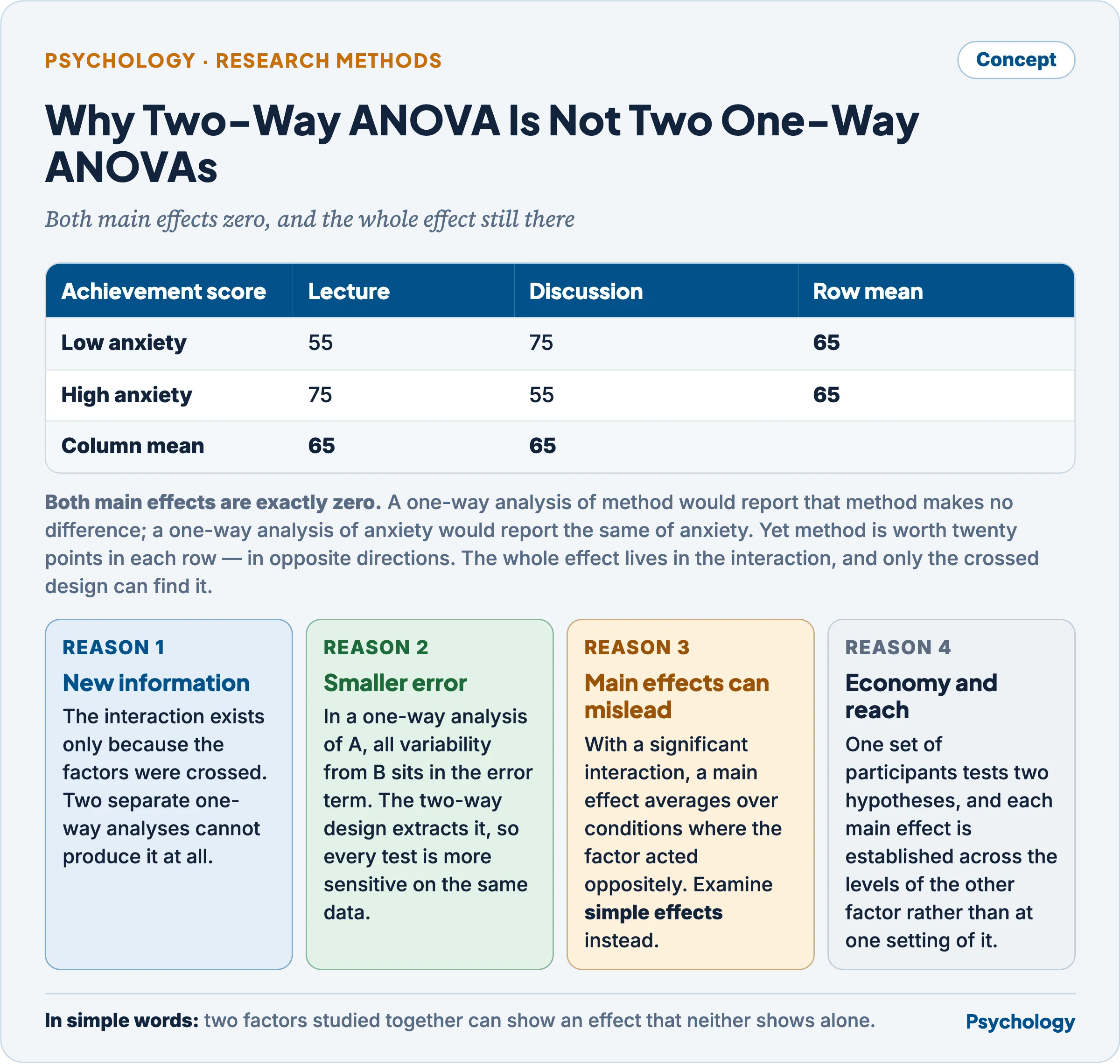
Neither one-way analysis would find anything here.

Both main effects are exactly zero: the two methods have identical column means and the two anxiety groups identical row means. A one-way analysis of method alone would report that method makes no difference, and a one-way analysis of anxiety alone would report the same of anxiety. Yet method matters enormously — it is worth twenty points in each row, in opposite directions. The whole effect lives in the interaction, and only the crossed design can find it. The correct follow-up is simple effects: discussion is superior for low-anxiety learners, lecture for high-anxiety learners. Reporting either main effect here would describe no one in the study, which is why a significant interaction is examined first and the main effects interpreted only if it is absent.

Effect size and statistical power

• Effect size is the magnitude of a difference or relation, in a metric that does not depend on sample size. For a difference between means it is Cohen’s d, the difference divided by the pooled standard deviation, with Cohen (1988) offering .2, .5 and .8 as rough markers of small, medium and large. For association it is r and r². For ANOVA it is eta-squared or partial eta-squared, with omega-squared the less biased estimate.
• Why it is needed. A significance test confounds magnitude with sample size: with a large enough sample an effect too small to matter reaches significance, and with a small sample an important effect fails to. “Significant” therefore answers a question about detectability, not about importance, and the effect size answers the question a reader actually has.
• Statistical power is the probability of rejecting a false null hypothesis — of detecting an effect that is really there. It equals 1 − β, where β is the probability of a Type II error. Four quantities determine it: the true effect size, the sample size, the significance level adopted, and whether the test is one- or two-tailed.
• Why it matters. Cohen (1962), reviewing a year of abnormal and social psychology, found that the median power to detect a medium effect was about .48 — a literature in which half the real effects present would be missed. Power analysis conducted before the study, to fix the sample size needed to detect the smallest effect worth finding, is the only effective response; computed afterwards from the obtained effect it adds nothing.
• The two connect to replication directly. An underpowered study not only misses real effects; when it does reach significance it must have obtained an unusually large estimate, so published effects from small studies are systematically overstated, and the replication attempt that follows is powered against an inflated target and fails.

Criticisms and limitations

• Null hypothesis significance testing answers a question nobody asked. The p value is the probability of data this extreme given that the null is true; what the investigator wants is the probability that the hypothesis is true given the data, and the two are not the same quantity. The null of exactly zero difference is also rarely a serious possibility in psychology, so rejecting it is a weak achievement.
• The .05 threshold is a convention with no principled basis, and treating it as a boundary between real and unreal converts a continuous measure of evidence into a dichotomy. Running analyses until one crosses it — selecting outcomes, covariates or subgroups after seeing the data — invalidates the stated error rate entirely.
• Assumption checking is performed inconsistently. Homogeneity of variance and independence matter most and are reported least, and independence is the failure that nothing repairs.
• Treating ordinal scores as interval is the discipline’s standing compromise. Rating-scale responses are analysed with means and t-tests on the assumption that the intervals are equal, which no evidence establishes.
• A significant F is often where the analysis stops. It establishes only that the means are not all equal, and without post hoc comparisons, effect sizes and a plot of the cell means it supports almost no substantive claim.
• No statistical technique repairs a defective design. An analysis cannot recover a comparison the design did not create, and the sophistication of the statistics applied is frequently inverse to the quality of the data they are applied to.