Correlation and Regression in Psychological Research

Application of statistical technique (correlation and regression).

Official Syllabus: Paper I · Unit 3 Research Methods

“Two variable organs are said to be co-related when the variation of the one is accompanied on the average by more or less variation of the other, and in the same direction.”

— Galton (1888)

Galton’s phrase “on the average” is the whole of it. A correlation is a statement about a tendency across many cases, not a claim about any one of them, and almost every misuse of these techniques consists in forgetting that. Correlation describes the relation symmetrically; regression turns it into an equation that predicts one variable from others and, in its multiple form, separates the contribution of each.

Correlation

Pearson’s product-moment correlation, r, developed by Pearson (1896) from Galton’s work, measures the strength and direction of the linear relation between two interval or ratio variables. It runs from −1 through 0 to +1, where the sign gives direction and the absolute value gives strength. Its square, the coefficient of determination, gives the proportion of variance in one variable accounted for by the other — an r of .40 accounts for 16 per cent, which is why a coefficient that sounds substantial often explains little.

Where the data are ranks or the relation is monotonic but not linear, Spearman’s rho is used; Kendall’s tau is the alternative for small samples with tied ranks. For two dichotomies the phi coefficient applies, and for one dichotomy against a continuous variable the point-biserial correlation, which is algebraically the same quantity as the independent-samples t.

Why a correlation does not establish a cause

A correlation between two measures is equally consistent with three accounts, and the coefficient cannot discriminate among them: the first causes the second, the second causes the first, or a third variable produces both.

The standard examination case has this structure. Where the number of students admitted to a college correlates highly with the incidence of violence, the readings available are:

• The relation is causal in the obvious direction — a larger intake produces crowding, anonymity and competition for scarce facilities, each of which plausibly raises conflict.
• The direction is reversed — a reputation for violence changes who applies and is admitted.
• A third variable produces both, which is the most probable account here. A growing town has more college places and more of every category of recorded incident, because both track population. Two series that each rise over time will correlate whether or not anything connects them, and the coefficient registers the shared trend.
• The ecological fallacy compounds it. The correlation is computed across institutions, and nothing whatever follows from it about any individual student at any of them.

The appropriate response is not a cautious phrasing but a change of design or analysis: hold the third variable constant by partial correlation where it has been measured, establish temporal order through longitudinal measurement, or find a source of variation in the presumed cause that is unrelated to the outcome.

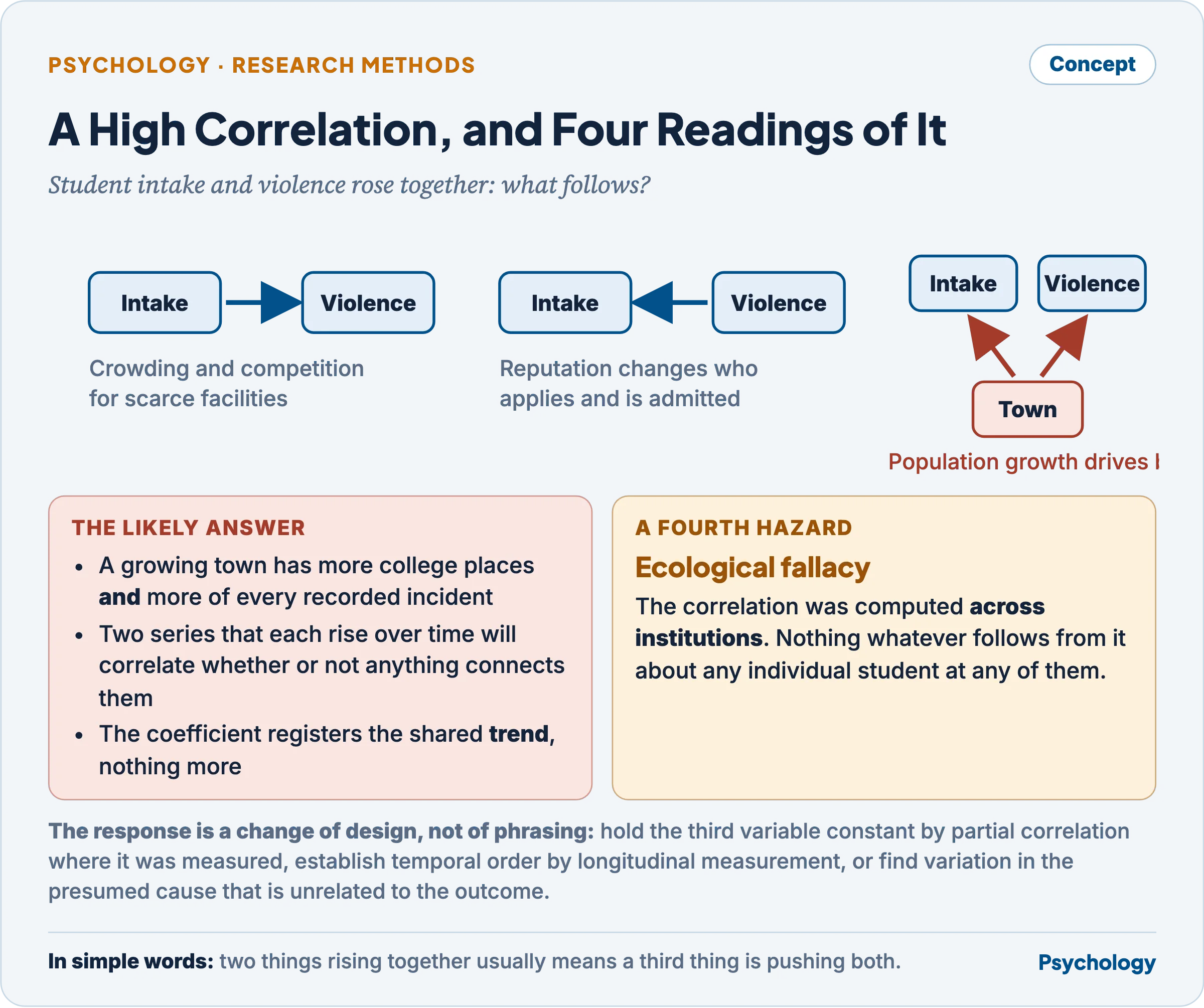
The coefficient cannot discriminate among them.

Further cautions

• Only linear relations are detected. A strong inverted-U relation — arousal and performance, for instance — returns an r near zero. Always inspect the scatterplot before the coefficient.
• Outliers distort it, particularly in small samples, where a single extreme pair can create or destroy a correlation.
• Restriction of range attenuates it. A selection test’s validity computed only on those admitted understates its real predictive power, because the low scorers who would have failed are absent from the sample.
• Aggregation inflates it. Correlations computed on group means are routinely far larger than the same correlation computed on individuals.
• Attenuation by unreliability. The observed correlation between two fallible measures is lower than the true correlation between the constructs, bounded by the square root of the product of their reliabilities.

Regression

Simple linear regression fits the equation Y = a + bX, where b, the regression coefficient, is the change in Y for a one-unit change in X, and a is the intercept. The line is fitted by least squares, minimising the sum of the squared vertical distances of the points from it, and b relates to the correlation by b = r × (sy ÷ sx).

Multiple regression fits Y = a + b1X1 + b2X2 + … , where each coefficient gives the effect of its own predictor with all the other predictors held constant. R, the multiple correlation, is the correlation between the observed and predicted scores, and R² the proportion of outcome variance accounted for by the predictors together. Adjusted R² corrects for the fact that R² can only rise as predictors are added, and is the figure to report.

When to choose multiple regression over the simple form

The choice is not a matter of sophistication; the conditions calling for the multiple form are specific.

• More than one variable plausibly predicts the outcome, and the question is their joint predictive power. Academic achievement is predicted by aptitude, study hours and home environment together, and a simple regression on any one of them overstates that one’s importance.
• A confound must be partialled out. To ask whether coaching improves performance net of prior ability, prior ability enters the equation as a second predictor, and the coefficient for coaching then estimates its effect among people of equal prior ability.
• The relative importance of predictors is at issue, which requires them in one equation on a common footing.
• Incremental validity is being tested — whether a new measure predicts anything beyond those already in use, read from the rise in R² when it is entered last.
• Moderation or mediation is to be modelled, through a product term or a sequence of equations.
• Prediction accuracy is itself the goal, since R² generally rises when a relevant predictor is added.

Against this, every predictor costs degrees of freedom and demands cases — a conventional minimum is ten to twenty per predictor — and predictors that are strongly intercorrelated bring the instability described below. Where one predictor is at issue and no confound needs removing, the simple form is the correct choice and by far the more interpretable one.

Ways of performing the analysis

• Simultaneous or standard entry — all predictors entered at once, each evaluated for what it adds over all the others. The default where no theory orders them.
• Hierarchical entry — predictors entered in blocks in an order fixed by theory, with the change in R² at each step reporting what that block adds. This is the method for testing incremental validity and for controlling covariates entered first.
• Stepwise entry — the algorithm adds or removes predictors by statistical criteria alone. It capitalises on chance in the particular sample, produces results that do not replicate, and is best avoided except in frankly exploratory prediction work.

Standardized and unstandardized coefficients

• The unstandardized coefficient b is in the original units: a one-unit rise in X is associated with a rise of b units in Y, other predictors held constant. It is the quantity used to write the prediction equation and compute a predicted score, it is interpretable in the real metric — rupees, minutes, items correct — and it is comparable across samples that used the same measures.
• The standardized coefficient β is in standard-deviation units: a one standard-deviation rise in X is associated with a rise of β standard deviations in Y. Being unit-free, it allows predictors measured on different scales to be compared for relative importance within one sample. In simple regression with a single predictor, β is numerically equal to r.
• A worked contrast. Predicting monthly income from years of education and from hours worked per week, b for education might be 3,200 rupees per year of schooling and b for hours 180 rupees per hour. Those two numbers cannot be compared, because a year and an hour are not the same size of step. The corresponding standardized coefficients of .42 and .26 can be compared, and they say that education is the stronger predictor in this sample.

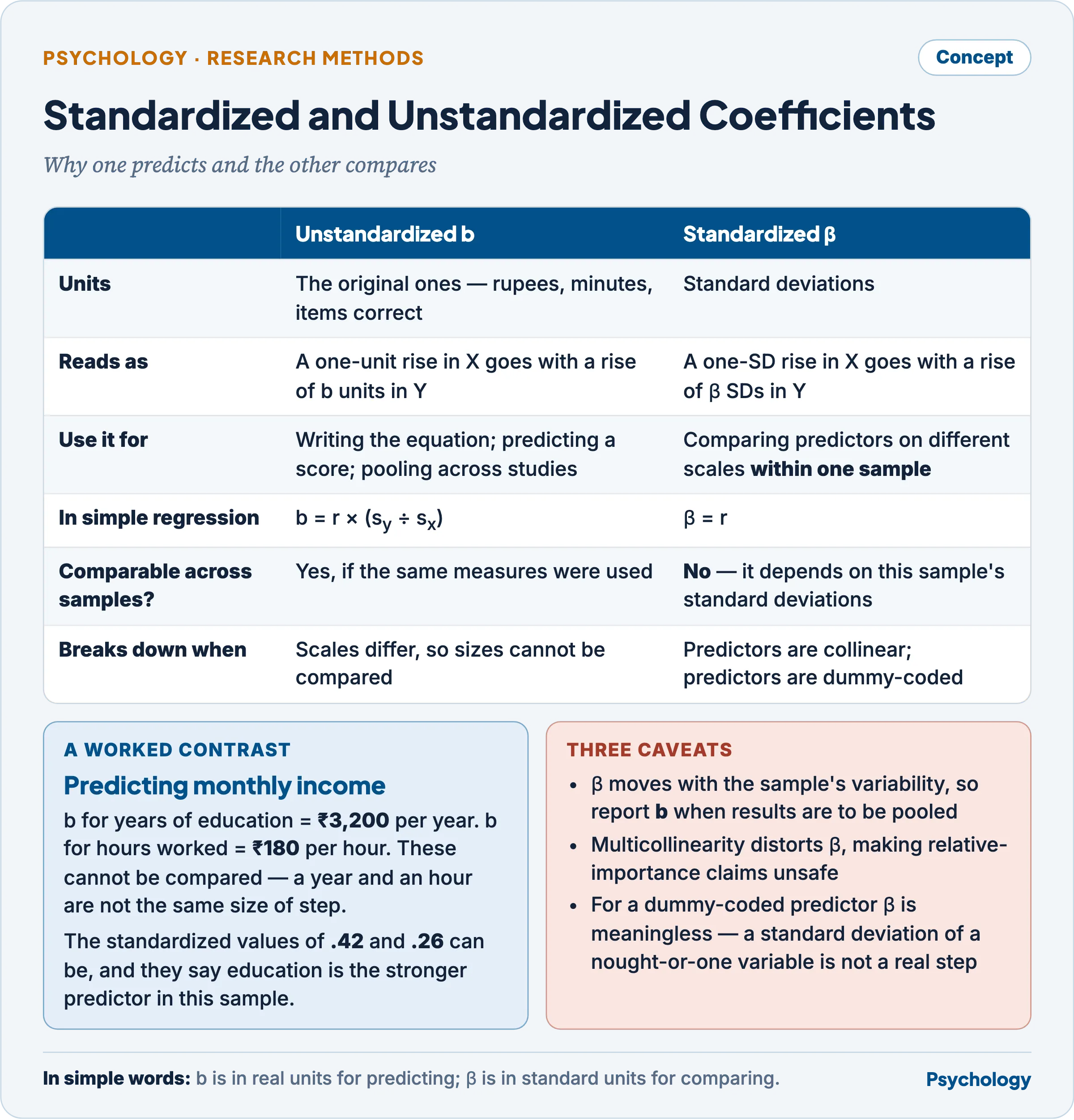
One is for predicting, the other for comparing.

• The caveats matter and are regularly ignored. β depends on the standard deviations in this sample, so it is not comparable across samples of differing variability — which is why b is reported when results are to be pooled across studies. β is distorted by multicollinearity, so relative-importance claims drawn from it are unsafe whenever predictors are correlated. And for a dummy-coded categorical predictor β has no sensible meaning, since a standard deviation of a nought-or-one variable is not a real step.

Assumptions, and what violation does

• Linearity — each predictor’s relation to the outcome is a straight line. Violation biases the coefficients and understates the relation. A plot of residuals against predicted values reveals it; transformation or a polynomial term repairs it.
• Independence of errors — residuals are uncorrelated with one another. Violation, common in time-series data and in clustered data such as pupils within schools, leaves the coefficients unbiased but severely understates the standard errors, so significance is grossly overstated. Multilevel modelling is the remedy.
• Homoscedasticity — residual variance is constant across the range of predicted values. Under heteroscedasticity the coefficients remain unbiased but the standard errors are wrong, so every significance test and confidence interval built on them is invalid. Transformation of the outcome, weighted least squares, or robust standard errors address it.
• Normality of residuals — required for inference in small samples; with large samples the central limit theorem makes the tests robust. Note that it is the residuals that must be normal, not the variables themselves.
• Absence of serious multicollinearity — predictors must not be near-perfectly intercorrelated. When they are, estimates become unstable, standard errors inflate, coefficient signs can reverse, and individual predictors appear non-significant although the overall R² is large and significant. The variance inflation factor and tolerance diagnose it; combining the redundant predictors, dropping one, or forming a composite is the usual answer. Singularity, where one predictor is an exact linear function of others, makes the solution impossible to compute at all.
• No unduly influential cases — a single outlier with high leverage can rotate the fitted line. Cook’s distance identifies them.
• Predictors measured without error — routinely violated in psychology, where every predictor is a fallible test score. The consequence is that an unreliable predictor’s coefficient is attenuated while a reliable one entered alongside it is inflated, so the apparent ranking of predictors partly reflects their reliabilities.

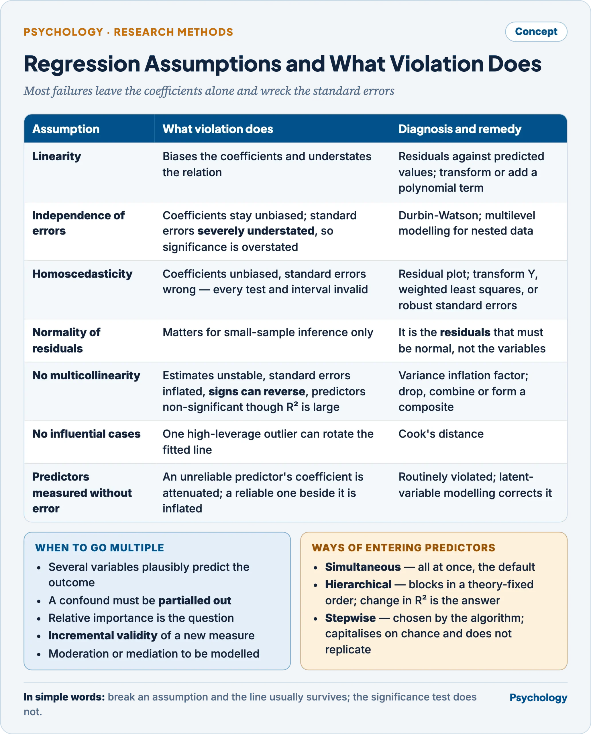
Most failures leave the coefficients alone and wreck the standard errors.

ANOVA or regression

The question of which is superior is best answered by denying the premise. Both are special cases of the general linear model, and an ANOVA is a regression in which the predictors are dummy-coded group memberships. The same data yield the same F.

What regression gains in practice is real, and that is the defensible content of the claim:

• It takes continuous predictors as they are. ANOVA requires categories, so a continuous variable must be split into groups — which discards information, lowers power, and makes the result depend on where the cut was placed.
• It handles any mixture of categorical and continuous predictors in one equation.
• It gives the magnitude and direction of each effect in interpretable units, where ANOVA’s F reports only that means differ somewhere.
• It predicts a score for a new case, which ANOVA does not attempt.
• It copes with unequal group sizes and with covariates without a separate procedure.
• It expresses non-linear and interaction terms explicitly, and allows predictors to be entered in a planned order so that incremental R² answers questions about what a variable adds.

What ANOVA retains is the natural expression of a designed factorial experiment: its output is organised as main effects and interactions, with post hoc machinery built for comparing specific means, and its conventions match how an experiment is reported. The honest statement is that ANOVA is the convenient form for experiments with categorical factors and regression the general form for everything else.

Criticisms and limitations

• Causal language attaches itself to regression coefficients. A coefficient is called an “effect” and read as what would happen if the predictor were changed. With observational data it is a conditional association, and “controlling for” a variable controls only the measured, reliably measured part of it.
• R² is over-read. It describes fit in this sample, rises mechanically with the number of predictors, and says nothing about whether the model would predict a new case. Cross-validation or a holdout sample is what answers that, and is rarely done.
• Stepwise selection remains in wide use despite producing variable sets that change with trivial changes in the data, and significance values that are not what they claim.
• The correlation-causation caution is taught universally and abandoned at the discussion section, where “associated with” becomes “leads to”. The remedy is design, not phrasing: without temporal ordering or an exogenous source of variation, no amount of statistical sophistication converts covariation into causation.
• Attenuation and restriction of range are seldom corrected for, so published correlations systematically understate relations among constructs while published regression coefficients misrank predictors by reliability.
• Linearity is assumed far more often than it is checked. A scatterplot costs nothing and is omitted routinely, and the relations psychology most cares about — arousal and performance, stress and health, practice and skill — are among those least likely to be straight.