

Official syllabusPaper II · Unit 1 · Psychological Measurement of Individual Differences
Characteristics and construction of standardized psychological tests – reliability.
Definition
“Reliability refers to the consistency of scores obtained by the same persons when they are reexamined with the same test on different occasions, or with different sets of equivalent items, or under other variable examining conditions.”
Anastasi and Urbina (1997)
Every test score mixes the attribute being measured with chance influences of the occasion, the items, the scorer and the testee. Reliability estimates how much of the score is the attribute, and because each method of estimating it counts a different influence as error, no single coefficient states “the” reliability of a test.
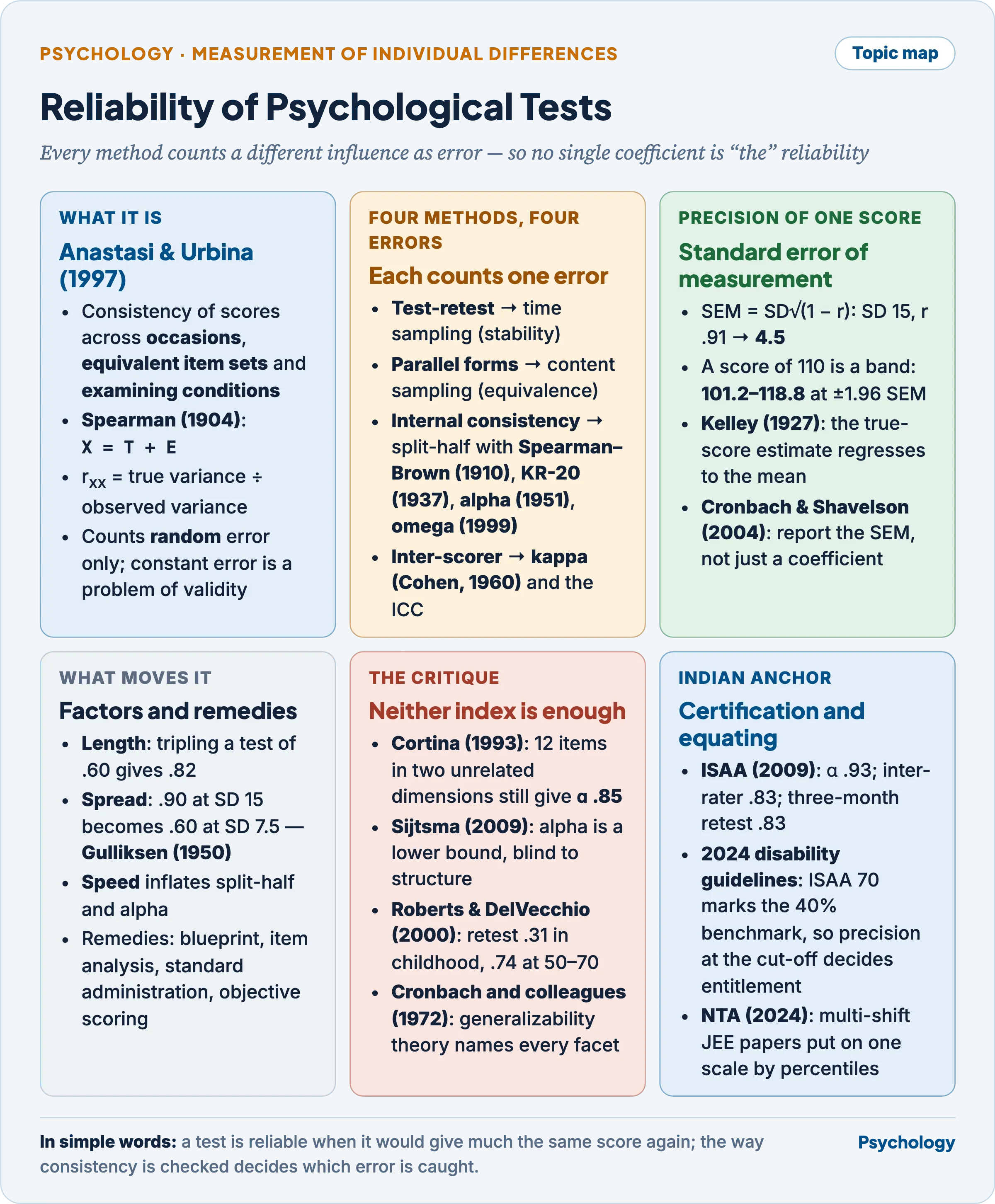
The four methods in the top-centre box each count a different influence as error, which is why the critique beneath them refuses to let any one coefficient stand for the rest.
Reliability among the characteristics of standardized psychological tests
- Reliability stands beside objectivity, validity and norms among the characteristics of a standardized test, all set out in Construction and Standardization of Psychological Tests. It comes first because a score that would change on a second sitting can serve no other purpose consistently.
The classical true-score model
- Spearman (1904) introduced the model on which classical theory rests: an observed score (X) is a true score (T) plus a random error (E), so X = T + E.
- Its assumptions are that errors average zero over endless parallel testings, are uncorrelated with true scores, and are uncorrelated across testings; every coefficient below inherits them.
- Observed variance then splits, σ²X = σ²T + σ²E, and the reliability coefficient is the true share: rxx = σ²T / σ²X = 1 − σ²E / σ²X.
- A coefficient of .91 means that 91 parts in 100 of the variation among testees are true variation; the index of reliability, the correlation of observed with true scores, is √rxx.
- Gulliksen (1950) codified the model, and Lord and Novick (1968) formalised the grades of equivalence that decide which coefficient is legitimate.
- Parallel: equal true scores and equal error variances.
- Tau-equivalent: equal true scores, unequal error variances; essentially tau-equivalent: true scores differing by a constant.
- Congeneric (Jöreskog, 1971): true scores linearly related, so items may reflect the attribute with unequal strength.
Sources of error variance
- Reliability concerns random error only. A constant error, like a scale set five kilograms heavy, leaves scores consistent and wrong — the distinction drawn in Sampling, Measurement and Methods of Data Collection (Paper I) and Validity of Psychological Tests.
- Anastasi and Urbina (1997) name four sources of random error, each isolated by a different method: time sampling, content sampling, content heterogeneity and scorer differences.
- Cronbach (1947) named the resulting coefficient of stability, coefficient of equivalence and coefficient of stability and equivalence, the last counting both time and content as error and so the smallest.
- Baumgartner (1989) separated relative reliability, consistency of persons’ rank order, from absolute reliability, consistency of the scores themselves, which the standard error of measurement expresses.
Methods of estimating reliability
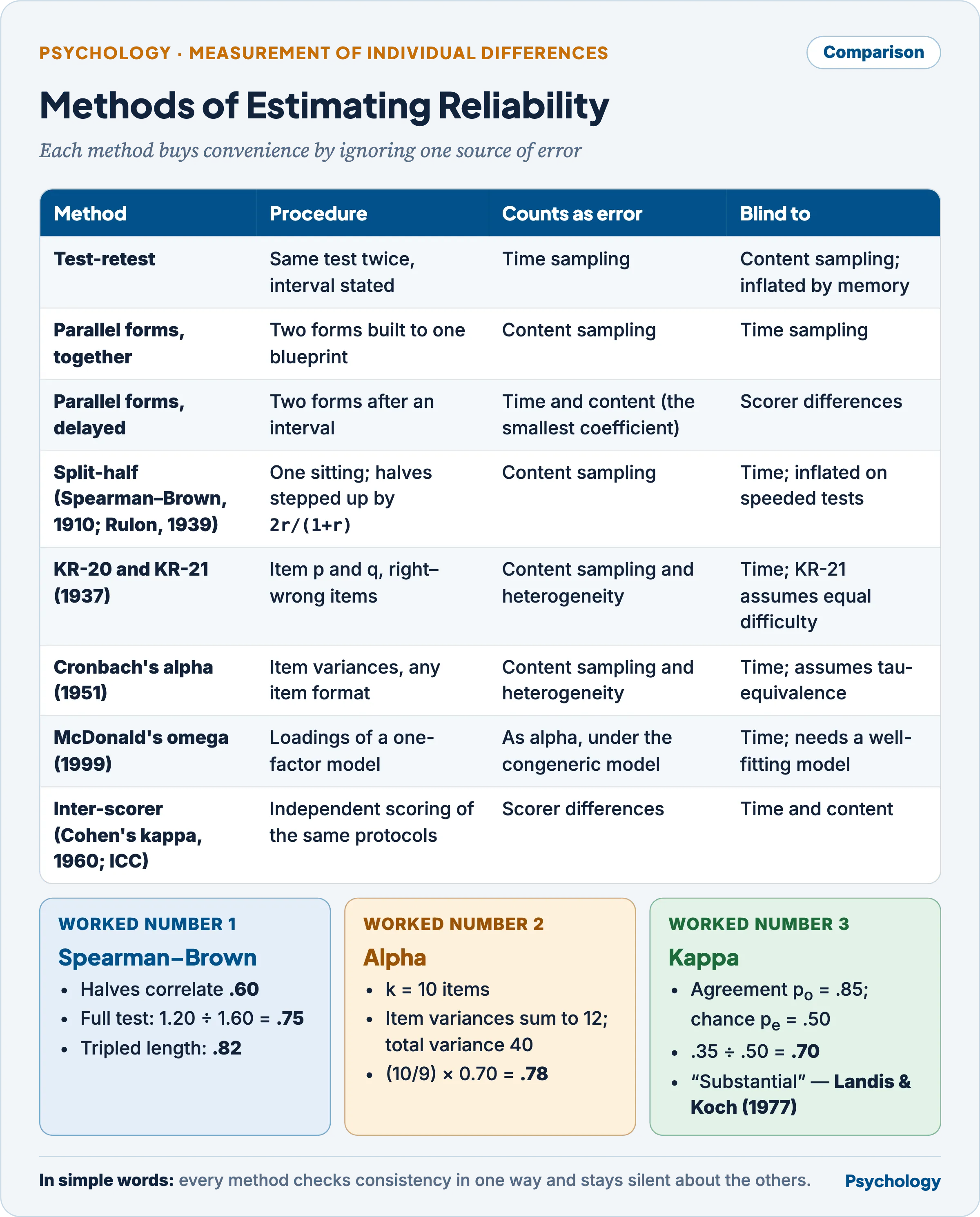
Read along a row: each method buys convenience by ignoring one source of error, and the last column names the source it ignores.
Test-retest reliability: the coefficient of stability
- The same test is given twice to the same group and the scores are correlated. The error counted is time sampling, and the interval must be stated because stability falls as it lengthens (Roberts and DelVecchio, 2000).
- A short interval lets testees remember answers, inflating the coefficient; a long one lets the trait itself change through development, learning or therapy, which the coefficient counts as error.
- It suits stable traits and aptitudes, not states, moods or tests whose first sitting alters the attribute (reactivity).
Parallel-form reliability: the coefficient of equivalence
- Two forms built to one specification are given to the same group and correlated: given together they count content sampling, given after an interval time and content as well (Cronbach, 1947).
- Gulliksen (1950) set the criteria two forms must meet before their correlation counts as a reliability.
- Psychological criteria: the same content specification, item format and number, instructions and time limits, and comparable validities.
- Statistical criteria: equal means, variances and intercorrelations, and equal correlations with any outside criterion, testable by the likelihood-ratio criterion of Wilks (1946).
- The method removes memory for particular items and supplies a form for retesting. It is costly, hard to make truly equivalent for personality and attitude content, and practice still transfers across forms.
Split-half reliability and the Spearman-Brown formula
- In one administration the test is split into comparable halves — odd against even items, or halves matched on content and difficulty — and the half-scores are correlated.
- A half-test samples content less well, so Spearman (1910) and Brown (1910), in one issue of the British Journal of Psychology, corrected it: rtt = 2rhh / (1 + rhh). Halves correlating .60 give 1.20 / 1.60 = .75.
- The general form, rkk = k·r / [1 + (k − 1)r], gives the effect of any change of length: tripling a test of .60 yields .82 (Spearman, 1910).
- Rulon (1939) published the formula of Flanagan (1937), which drops the assumption of equal half-variances: rtt = 1 − σ²d / σ²X, d being the difference between half-scores. Guttman (1945) gave the same coefficient as λ4.
- Each split yields a different value, and on a speeded test both halves share the number of items reached, inflating the coefficient; separately timed halves or a retest are needed (Anastasi and Urbina, 1997). The speed-power typology is in Types of Psychological Tests.
Internal consistency: Kuder-Richardson formulas and Cronbach’s alpha
- Kuder and Richardson (1937) removed the arbitrary split by working from item statistics, the older literature’s rational equivalence.
- KR-20 = [k/(k − 1)] × [1 − Σpq / σ²X] for right-wrong items, p being the proportion passing an item and q = 1 − p.
- KR-21 = [k/(k − 1)] × [1 − M(k − M) / (k·σ²X)] needs only the mean because it assumes equal difficulty, and underestimates when difficulties vary.
- Hoyt (1941) reached the same value by analysis of variance, and Guttman (1945) derived the general formula as λ3, third of six lower bounds to reliability.
- Cronbach (1951) generalised KR-20 to multi-point items and proved coefficient alpha to be the mean of all possible split-half coefficients: α = [k/(k − 1)] × [1 − Σσ²i / σ²X].
- Ten items whose variances sum to 12, with a total variance of 40, give α = (10/9) × 0.70 = .78.
- It needs one sitting and no arbitrary split, and suits any item format; its limitations are taken up below.
McDonald’s omega
- McDonald (1999) computed reliability from a one-factor model of the items: omega = (Σλ)² / [(Σλ)² + Σθ], λ being the item loadings and θ the item error variances.
- It assumes only the congeneric model and equals alpha under tau-equivalence; Dunn, Baguley and Brunsden (2014) recommend reporting it in place of alpha, and McNeish (2018) lists it among the better alternatives.
- It is only as sound as the factor model’s fit, needs larger samples, and for multidimensional scales is computed per subscale or as omega hierarchical; the factor model is in Factor Analysis and Multivariate Techniques (Paper I).
Inter-scorer reliability
- Where scoring involves judgement — essays, projective protocols, observation schedules, clinical ratings — scorers score the same protocols independently, and the error counted is scorer differences.
- Cohen (1960) removed chance agreement from raw percentage agreement with kappa: κ = (po − pe) / (1 − pe).
- Agreement on 85 of 100 protocols, where chance predicts 50, gives κ = .35 / .50 = .70, “substantial” on the benchmarks of Landis and Koch (1977).
- Continuous ratings take the intraclass correlation (ICC). Shrout and Fleiss (1979) distinguished six forms, and choosing absolute agreement over consistency makes a uniformly lenient scorer count as error.
- Koo and Li (2016) read an ICC below .50 as poor, .50–.75 moderate, .75–.90 good and above .90 excellent.
The standard error of measurement
- A coefficient describes a test in a group; the standard error of measurement (SEM) describes the precision of one person’s score: SEM = SD × √(1 − rxx).
- An intelligence test with SD 15 and reliability .91 has SEM = 15 × .30 = 4.5. Around 110, 105.5–114.5 holds the true score two times in three, and 101.2–118.8 (±1.96 SEM) 95 in 100 (Cronbach and Shavelson, 2004).
- Nunnally (1978) stated the consequence: “Even with a reliability of .90, the standard error of measurement is almost one-third as large as the standard deviation of the test scores.”
- Kelley (1927) regressed the estimated true score towards the group mean, T′ = M + rxx(X − M). With mean 100 and reliability .91, an observed 130 estimates 127.3, below a giftedness cut-off of 130.
- Gulliksen (1950) ranked four standard errors for any reliability below 1: estimating the true score, SD√[r(1 − r)]; measurement, SD√(1 − r); predicting a parallel-form score, SD√(1 − r²); and substitution of one form’s score for the other’s, SD√[2(1 − r)].
- The standard error of the difference, SD√(2 − r1 − r2) (Anastasi and Urbina, 1997), governs profiles and change. Two T-score subtests with reliabilities .90 and .80 give 5.5, so gaps under about 11 points are not interpretable.
- Green (1950) showed that the SEM can stay constant across groups whose coefficients differ widely, and Cronbach and Shavelson (2004) called it “the most important single piece of information to report regarding an instrument, and not a coefficient.”
- One SEM assumes equal precision at every level; precision that varies with ability is the test information function of Item Response Theory (Paper I).
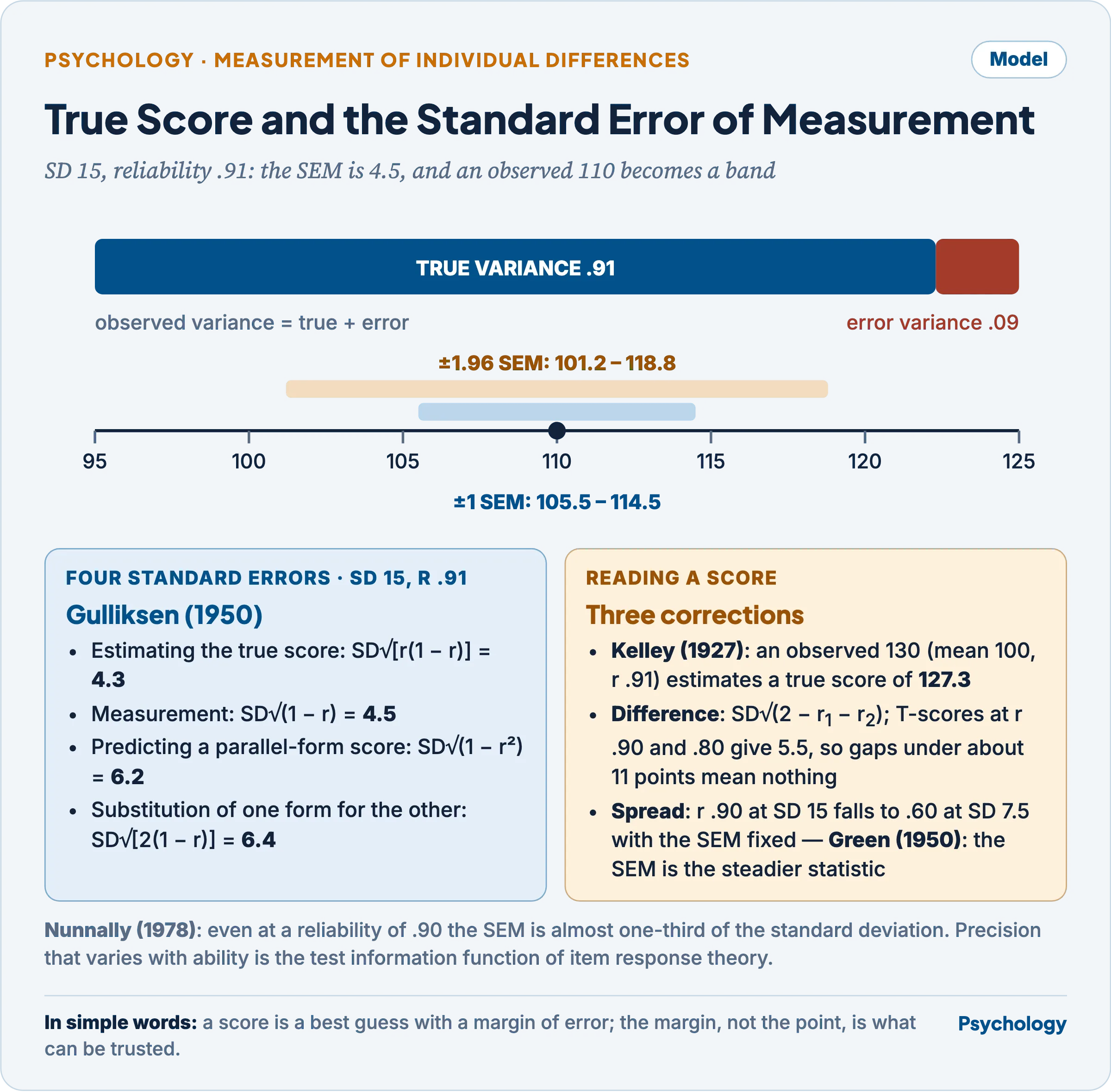
The same 110 is a band, not a point, and the band widens as the score is put to harder uses.
Factors affecting reliability
- Test length. More items sample the domain better, with diminishing returns: alpha’s rise with length is curvilinear and levels off before about 19 items (Komorita and Graham, 1965, cited by Cortina, 1993).
- Group heterogeneity. With the SEM fixed, reliability .90 in a population of SD 15 falls to .60 in a selected group of SD 7.5, by the relation set out by Gulliksen (1950), r′ = 1 − (σ²/σ′²)(1 − r).
- Hedge, Powell and Sumner (2018) found retest reliabilities of 0 to .82 for seven classic tasks such as Stroop and flanker: low between-person variance, which makes the effects robust, starves the coefficient. A flanker cost score reached .40, its components .74 and .66.
- Item difficulty and discrimination. Items that nearly everyone passes or fails add no variance, as worked out in Item Analysis and Item Validation.
- Speededness inflates split-half and internal-consistency coefficients, not retest or alternate-form ones.
- Other sources. The interval, guessing on true-false items, ambiguous wording, variable administration, subjective scoring, and testee fatigue, anxiety or motivation all alter error variance.
- The level required. Nunnally (1978) accepted .70 in early research and .80 in basic research, and for decisions about individuals called .90 “the minimum that should be tolerated”; Lance, Butts and Michels (2006) showed the universal “.70 rule” misreports him.
Methods for making a psychological test reliable in construction
- Define the construct and write items from a blueprint, so that they sample the domain evenly (Construction and Standardization of Psychological Tests).
- Lengthen with items of the same kind. The Spearman-Brown factor n = rd(1 − ro) / [ro(1 − rd)] shows that raising .60 to .80 needs 2.67 times the length, about 54 items from 20.
- Item-analyse a try-out: drop items with low or negative corrected item-total correlations, near-zero variance or extreme difficulty, and revise weak distractors.
- Write unambiguous items and instructions, and prefer four-option items to true-false to cut guessing.
- Standardise administration: instructions, time limits, conditions and trained examiners.
- Objectify scoring: keys, rubrics with anchor scripts, scorer training, double scoring with kappa or the ICC monitored, and machine scoring.
- Make it a power test unless speed is the construct, and estimate speeded tests by retest or separately timed halves.
- Estimate on a sample as varied as the population of use and re-estimate in each new one, since reliability “can only be discussed in relation to a particular sample of persons” (Cronbach, 1947).
- Retest with alternate forms, after an interval long enough to blunt memory and short enough to hold the trait constant.
- Aggregate raters or occasions, using a decision study to set how many, and give the SEM band with every score.
Generalizability theory
- Cronbach, Gleser, Nanda and Rajaratnam (1972) replaced the single error term with named facets — items, occasions, raters, tasks — and the true score with a universe score, the mean over all admissible observations.
- A G study estimates by analysis of variance a component for persons, each facet and each interaction; a D study uses them to design measurement, such as how many raters and tasks an essay score needs.
- It gives a generalizability coefficient for ranking and a dependability index (Φ) for decisions against a cut-off; alpha and the ICC are its one-facet special cases (Shrout and Fleiss, 1979).
- Cronbach’s late judgement: “Coefficients are a crude device that does not bring to the surface many subtleties implied by variance components” (Cronbach and Shavelson, 2004).
- Its demands — crossed designs, large samples, randomly sampled facets — keep it largely within big assessment programmes.
Critical evaluation of internal consistency and stability coefficients
| Internal consistency (split-half, KR-20, alpha, omega) | Stability (test-retest) | |
|---|---|---|
| Error counted | Content sampling and heterogeneity, at one moment | Time sampling across an interval |
| Administrations | One | Two, with attrition between |
| Inflated by | Speed; redundant items; length; correlated errors | Memory and practice at short intervals |
| Deflated by | Multidimensionality; unequal loadings (alpha) | Genuine change; reactivity |
| Suited to | Power tests; decisions on one occasion | Traits and aptitudes; prediction over time |
| Unsuited to | Speeded tests | States, moods, fast-developing abilities |
- Cronbach (1947) gave the verdict before either became routine: “No one of these is the ‘right’ coefficient. They measure different things, and each is useful.”
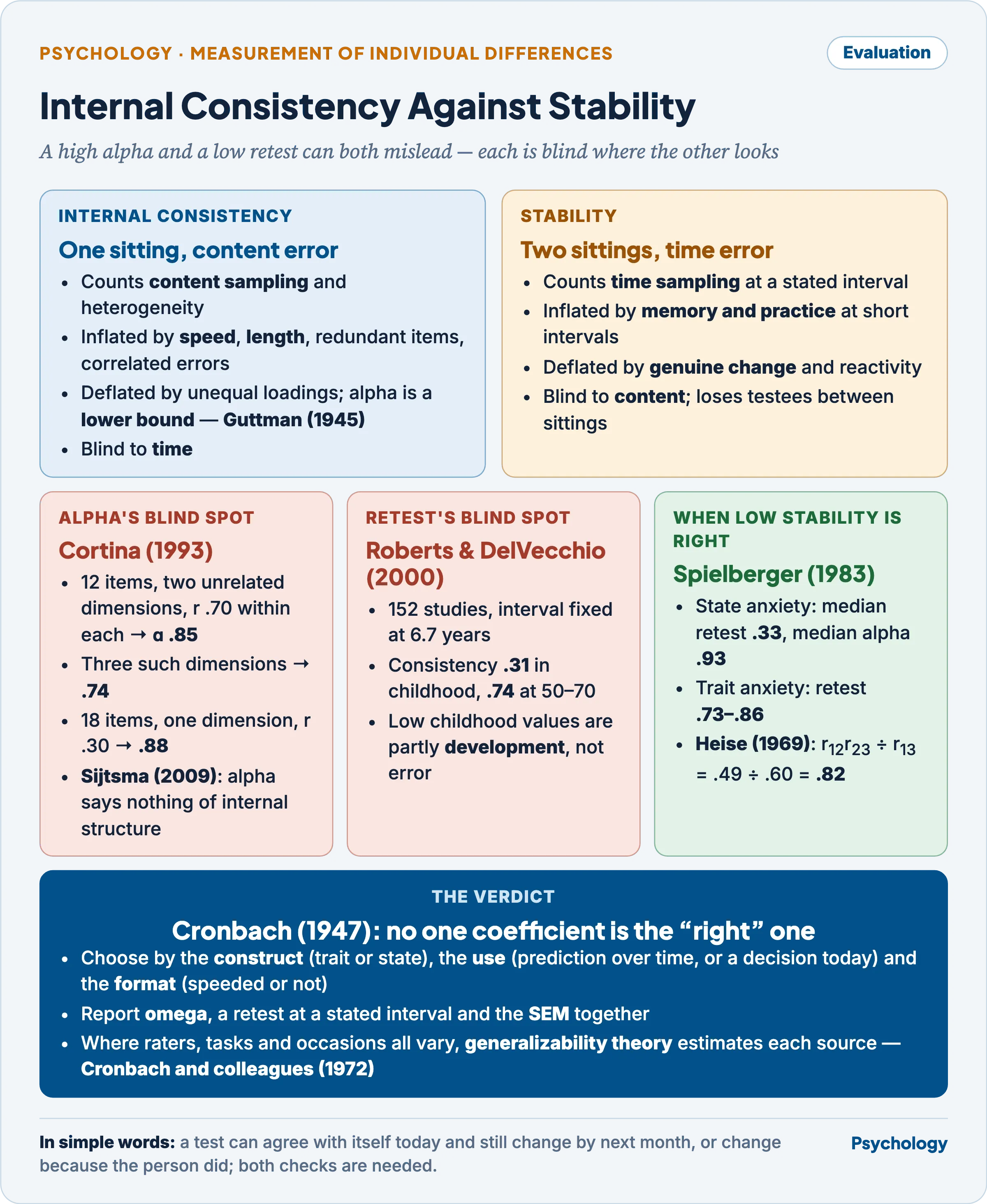
A high alpha can come from length or from several unrelated dimensions, and a low retest from real change: neither number explains itself.
- Alpha is not unidimensionality. Cortina (1993) found that 12 items forming two unrelated dimensions, correlating .70 within each, gave α = .85, and three dimensions .74; past 14 items, two dimensions correlating only .30 within each still exceeded .70.
- Sijtsma (2009) showed alpha unrelated to internal structure and, as a lower bound, possibly tenths below the reliability. The bound holds only for uncorrelated errors: shared wording or method inflates alpha, while unequal loadings deflate it (Dunn, Baguley and Brunsden, 2014).
- Loevinger (1954) named the attenuation paradox: past a point, making items more alike raises reliability while narrowing the construct and lowering validity, so a very high alpha signals redundancy.
- Retest confounds change with error. Roberts and DelVecchio (2000), pooling 3,217 coefficients from 152 longitudinal studies at a fixed 6.7-year interval, found consistency of .31 in childhood, .54 in college, .64 at 30 and .74 at 50–70.
- Much of the childhood “unreliability” is development, not error.
- For a state measure, low stability is evidence of validity. State anxiety on the State-Trait Anxiety Inventory had a median retest correlation of .33 against a median alpha of .93, while trait anxiety retested at .73–.86 (Spielberger, 1983).
- Heise (1969) separated reliability from stability with three waves: reliability = r12·r23 / r13. With r12 = r23 = .70 and r13 = .60 it is .82, above every retest correlation, on the assumption of equal reliability at each wave.
- Memory and practice inflate short-interval coefficients, testing can itself change the trait, and the interval is arbitrary, so no test has a single retest reliability.
- The two are complements, chosen by the construct (trait or state), the use (prediction over time, or a decision today) and the format (speeded or not). The defensible set is omega, a dated retest and the SEM, with generalizability theory where several facets operate.
- How reliability caps validity, and the correction for attenuation, belong to Validity of Psychological Tests.
Indian context
- Indian Scale for Assessment of Autism (ISAA) (Ministry of Social Justice and Empowerment, 2009) — built at the National Institute for the Mentally Handicapped, Secunderabad (1984; now NIEPID), to certify autism: 40 items in six domains, each rated 1–5 from observation, parent interview and testing.
- On 1,123 participants aged 3–22 from ten centres the manual reports alpha .93 in the autism group, inter-rater .83 on 67 children and three-month retest .83 on 120 (National Institute for the Mentally Handicapped, 2009).
- That inter-rater index is a Pearson correlation, blind to one rater’s systematic leniency; an absolute-agreement ICC is the stricter test where a cut-off decides entitlement.
- Mukherjee, Malhotra, Aneja, Chakraborty and Deshpande (2015), in 90 high-risk Delhi children aged 2–9, found retest .93–.99 and inter-rater .99, but acceptable construct validity in two of six domains and κ = .14 against the Childhood Autism Rating Scale.
- Guidelines for assessing the extent of specified disabilities (Department of Empowerment of Persons with Disabilities, notified 12 March 2024 under the Rights of Persons with Disabilities Act, 2016) — after diagnosis with the AIIMS-modified INCLEN tool, the ISAA score sets disability from age six.
- Bands: 70–106 mild (40–59 per cent), 107–153 moderate (60–79), above 153 severe (Gazette of India, 2024).
- It operationalises the cut-score decision: 40 per cent is the Act’s benchmark disability, so a child within one SEM of 70 may fall either side of an entitlement (Gazette of India, 2024).
- Chatterjee and Sahay (2024) noted that no rule assigns a percentage within a band.
- National Testing Agency (Ministry of Education, 2017) runs JEE (Main) in shifts with papers “of a similar nature in content” chosen “without knowledge of the difficulty level” — 10 shifts in Session 1 of 2024 (NTA, 2024).
- Such forms are parallel in content, not statistically, so candidates are randomly allotted to shifts and raw scores converted to within-shift percentile scores, a procedure set by experts from ISI, IISc and the IITs in 2018 (NTA, 2024).
- The principle is equating: Gulliksen’s equal-means criterion, unmet by construction, is imposed statistically, with percentile scales treated in Test Norms and Norm-Referenced Measurement.
Previous Year Questions
- 2025What are the different methods of estimating internal consistency reliability? Explain their strengths and limitations.
- 2021Describe the different methods for making a psychological test reliable.
- 2011Critically evaluate internal consistency and stability coefficients as indices of reliability.
- 2002Elucidate the nature of individual differences. Describe the methods of validity and reliability.