

Official syllabusPaper II · Unit 1 · Psychological Measurement of Individual Differences
Characteristics and construction of standardized psychological tests – item analysis.
Definition
“The computation and examination of any statistical property of examinees’ responses to an individual test item.”
Crocker and Algina (1986)
A test is only as good as its items, and item analysis is the stage of construction at which try-out data decide which items survive and which are rewritten or dropped. Item validation asks the harder question — whether each surviving item measures the intended attribute rather than something merely correlated with it — and it is where classical statistics, scaling, item response theory and factor analysis meet.
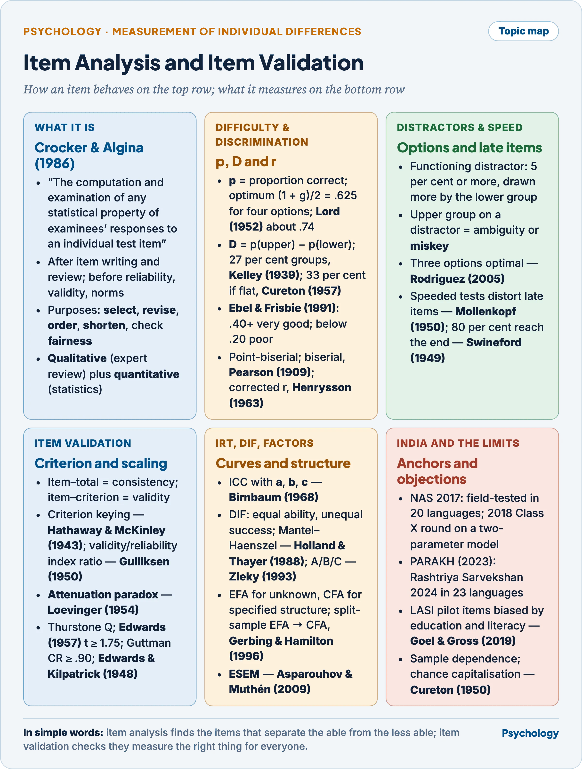
The top row asks how an item behaves; the bottom row asks what it measures, and whether it measures it equally for everyone.
Item analysis in the construction of standardized psychological tests
- Item analysis evaluates each item from try-out data after item writing and expert review, and before reliability, validity and norms (Construction and Standardization of Psychological Tests).
- Its purposes:
- Selection of items that measure the attribute, and revision of those whose wording or options misfire.
- Ordering and spread by difficulty, as Binet and Simon (1905) arranged the thirty items of their scale in ascending difficulty after trying them out on children.
- Economy — a shorter test of better items can be more reliable and valid than a longer one.
- Fairness — finding items that behave differently for groups of equal ability.
- Qualitative item analysis is expert judgement of content, wording, key and cultural load; quantitative item analysis, the statistics of difficulty, discrimination, distractors and validity. Neither replaces the other.
- Zubin (1934) proposed selecting items by internal consistency.
Item difficulty
- Item difficulty (p) is the proportion of testees answering correctly — really an index of easiness. For a personality or attitude item the same statistic is the endorsement index, the proportion agreeing.
- Percentages are unequal units, so p is often rescaled as the delta index, Δ = 13 − 4z (z the normal deviate of p): 84 per cent passing gives Δ = 9, 16 per cent Δ = 17 (Holland and Thayer, 1985).
- The optimal difficulty depends on guessing.
- Without guessing, p = .50 maximises item variance and so the number of passer–failer distinctions.
- With guessing, the working rule puts it midway between chance and 1.00 — (1 + g)/2, or .625 for four options.
- Lord (1952) showed the optimum for reliability lies a little higher: about .74 for four options, .70 for five, .77 for three, .85 for true–false.
- Purpose sets the spread: ranking across the range needs difficulties spread around the optimum; selection at a cut-off needs items concentrated near the cut-off’s difficulty.
- p belongs to the item and the try-out sample — easy for one group, hard for another — the sample-dependence that Item Response Theory (Paper I) removes.
Item discrimination
The discrimination index and the 27 per cent groups
- Item discrimination is the degree to which an item separates testees high on the attribute from those low on it, total score serving as the working criterion.
- The discrimination index D = p(upper) − p(lower), running from +1.00 through 0 to −1.00.
- Kelley (1939) showed that upper and lower groups of 27 per cent of a normal distribution are optimal; Cureton (1957) showed the optimum becomes 33 per cent for a flat, rectangular distribution.
- Ebel and Frisbie (1991): D of .40 and above, very good; .30 to .39, reasonably good; .20 to .29, marginal, usually needing improvement; below .20, poor.
- D is easily hand-computed but ignores the middle 46 per cent (Kelley, 1939) and is capped by difficulty: an item everyone passes cannot discriminate.
Point-biserial, biserial and the corrected item–total correlation
- The point-biserial correlation (r-pbis) is the product-moment r between a right–wrong item score and the total, treating the item as a true dichotomy; its ceiling is below 1 — about .80 at p = .50 for a normal total — and falls as p moves away.
- The biserial correlation (Pearson, 1909) assumes a normal ability beneath the pass–fail split. It is always larger than the point-biserial, less tied to p, and can exceed 1 when normality fails.
- An item inside the total correlates partly with itself, most in short tests. Henrysson (1963) derived corrections for this overlap; the corrected item–total correlation uses the total of the remaining items.
- Rating-scale items use the Pearson r with the total.
Distractor analysis
- Distractor analysis tabulates how many testees in the upper and lower groups chose each wrong option, or distractor, of a multiple-choice item.
- A functioning distractor draws more of the lower group than the upper and a noticeable share overall; one chosen by fewer than 5 per cent is non-functioning (Haladyna and Downing, 1993).
- Three diagnostic patterns:
- an option no one chooses is dead weight, to be replaced;
- a distractor favoured by the upper group signals an ambiguous stem or a second defensible answer;
- a key chosen by fewer of the upper group than a distractor signals a miskey.
- Rodriguez (2005), synthesising eighty years of research, found three options optimal: two good distractors cost no quality and allow more items per hour, though deleting distractors at random lowers reliability.
Item analysis on speed tests
- A pure speed test has items so easy that errors are negligible, so score reflects number attempted; a pure power test allows ample time, so score reflects difficulty mastered (Gulliksen, 1950). Most aptitude tests are mixtures.
- Late items in a timed test are distorted, because a testee who never reached an item is counted as failing it: p is underestimated, and discrimination inflated, since the abler testees are also the faster.
- Mollenkopf (1950) found the proportion right among those attempting, the delta index and the biserial r all behaving undesirably for items placed late in a speeded test.
- Oshima (1994), simulating speeded tests under item response theory, found item discrimination and difficulty overestimated and guessing underestimated.
- Remedies:
- generous try-out time — a test counts as unspeeded when about 80 per cent reach the last item (Swineford, 1949) and virtually all reach three-quarters of it (Swineford, 1956);
- “not reached” scored apart from “wrong”, with item statistics computed only on those who reached the item;
- no odd–even reliability for a speeded test (Reliability of Psychological Tests).
Item analysis of an aptitude test: a worked try-out
For a sixty-item numerical, verbal and spatial aptitude test for administrative trainees:
- Blueprint and pool — define each aptitude; write about one and a half times the final number of items.
- Qualitative review — experts check keys, ambiguity, coverage and cultural or linguistic load; translations are checked before try-out.
- Try-out — 370 testees resembling future candidates, with time generous enough to make it a power test.
- Groups — rank by total within each sub-test, since an item is judged against its own aptitude; take the top and bottom 27 per cent, 100 each.
- Statistics — p, D, corrected item–total r and the option-by-group distractor table.
- Decisions — keep, revise, rekey or discard by the rules above.
- Fairness — Mantel–Haenszel DIF by medium of instruction, gender and region where group sizes allow.
- Assembly and cross-validation — build the final form to blueprint and difficulty target; confirm retained items on a fresh sample.
Six items from a hypothetical try-out (key in bold; p from the two extreme groups):
| Item | Upper 100 (A/B/C/D) | Lower 100 (A/B/C/D) | p | D | r (corrected) | Decision |
|---|---|---|---|---|---|---|
| 1 Number series, key B | 4/82/8/6 | 18/42/22/18 | .62 | .40 | .41 | Keep: near the optimum; distractors draw the lower group |
| 2 Analogy, key C | 1/0/97/2 | 5/2/89/4 | .93 | .08 | .09 | Discard, or keep only as a warm-up item |
| 3 Data interpretation, key A | 28/6/12/54 | 26/30/28/16 | .27 | .02 | .03 | Check the key: option D draws the upper group |
| 4 Spatial, key D | 14/0/10/76 | 34/0/30/36 | .56 | .40 | .38 | Keep; replace option B, chosen by no one |
| 5 Verbal reasoning, key B | 30/18/26/26 | 24/33/21/22 | .26 | −.15 | −.14 | Discard: the abler testees are misled |
| 6 Hard numerical, key C | 20/18/44/18 | 28/30/12/30 | .28 | .32 | .29 | Keep: hard but discriminating, for the top of the range |
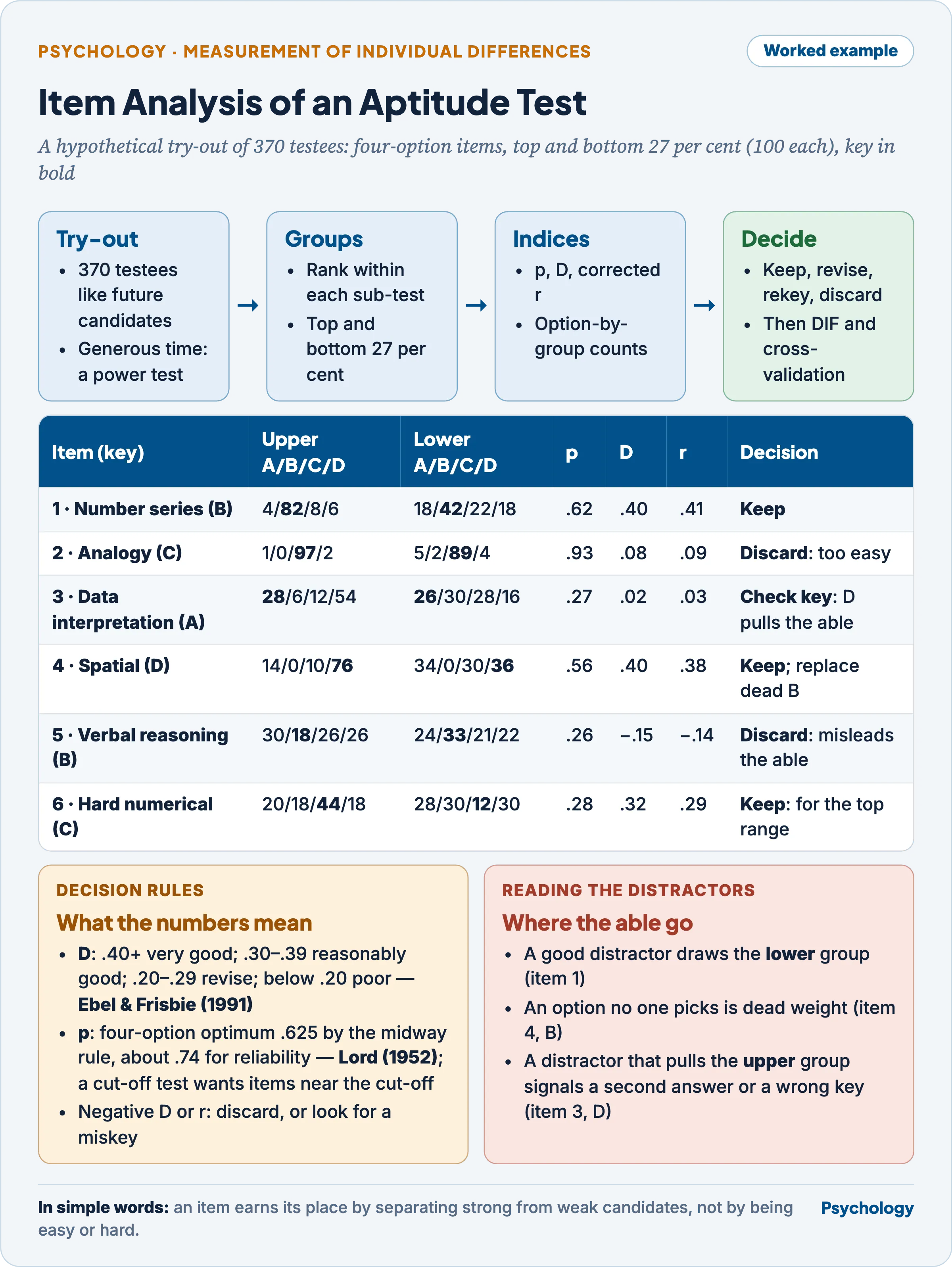
Difficulty alone never condemns an item: item 6 is hard and kept, item 2 easy and dropped, because only one separates the able from the less able.
Item validity and item validation
Internal consistency against an external criterion
- Item validity is an item’s relation to an external criterion — training grades, job ratings, diagnosis. Its relation to the test’s own total is evidence of internal consistency only.
- The two build different tests: item–total selection yields a homogeneous test, item–criterion selection a predictive test of mixed content.
- Hathaway and McKinley (1943) kept MMPI items that separated clinical groups from normal respondents whatever their content — empirical criterion keying (Validity of Psychological Tests).
- Gulliksen (1950) proposed maximising test validity by selecting items with a high ratio of the item-validity index (item SD × item–criterion r) to the item-reliability index (item SD × item–total r).
- Loevinger (1954) named the attenuation paradox: pushing internal consistency past a point narrows content and lowers validity. Clark and Watson (2019) treat empirical, internal-consistency and item-response selection as strategies to combine.
- Cureton (1950) — the demonstration that item validities must be cross-validated.
- Twenty-nine students “took” an 85-item test of numbered tags shaken in a cocktail shaker; a tag landing number-up scored “plus”.
- The 24 tags kept for their apparent relation to grade-point average gave a validity of .82 — against .23 for a real vocabulary test — with a KR-20 of −.06.
- His verdict on validities from the selecting sample: “Baloney!” They capitalise on chance and must be recomputed on a fresh sample: cross-validation.
- Limitation: a deliberate reductio on a tiny sample; real shrinkage depends on sample size and the number of items screened.
Item validation in psychometric scaling
- Psychometric scaling places statements and persons on one continuum; item validation in scaling is the evidence that each item belongs on it, at its assigned position, and measures nothing else (procedures in Measurement of Attitudes, Paper I).
- Thurstone (1928) — judges’ scale value, the Q index of ambiguity, and the criterion of irrelevance: a statement endorsed at every position is off the continuum.
- Likert (1932) — item–total correlation; Edwards (1957) retained statements whose means differ between the top and bottom 25 per cent with t of at least 1.75.
- Guttman (1944) — items validated as a set by cumulative pattern, with reproducibility of at least .90.
- Edwards and Kilpatrick (1948) fused all three in the scale-discrimination technique, after showing that statements with comparable Thurstone scale and Q values can differ greatly in power to separate favourable from unfavourable respondents.
- The steps:
- Define the continuum; write a pool balanced in direction.
- Judge relevance by expert ratings, quantified by the content validity ratio of Lawshe (1975).
- Try out on the target population.
- Compute endorsement, item–total r or criterion-group t, and ambiguity where judges are used.
- Check dimensionality by scalogram or item factor analysis.
- Validate externally by known-groups contrast or a criterion.
- Screen for DIF across languages and groups.
- Cross-validate; then estimate reliability and norms.
- In item response theory, item validation becomes item fit: an item is kept when its responses follow the model’s curve.
Item characteristics under item response theory and differential item functioning
- The item characteristic curve (ICC) gives the probability of success as a function of ability, θ, with three parameters (Birnbaum, 1968): b, difficulty, the θ at the curve’s midpoint; a, discrimination, the slope there; c, the lower asymptote set by guessing.
- They parallel p, D and the chance level but, when the model fits, do not depend on the sample’s ability spread (Item Response Theory, Paper I).
- Differential item functioning (DIF) exists when testees of equal ability from different groups have different probabilities of success on an item. Uniform DIF shifts one group’s curve sideways; non-uniform DIF changes its slope, so the curves cross.
- The Mantel–Haenszel procedure (Mantel and Haenszel, 1959), adapted to items by Holland and Thayer (1988), matches groups on total score, compares the odds of success at each score level, and pools them into one odds ratio expressed as MH D-DIF.
- Zieky (1993) set out three classes: A, negligible (below 1 in absolute value, or not significant); C, large (at least 1.5 and significantly above 1); B, the rest. C items are reviewed and may be dropped.
- Logistic regression (Swaminathan and Rogers, 1990) detects non-uniform DIF more powerfully than the Mantel–Haenszel statistic, and uniform DIF as powerfully.
- DIF is a flag, not proof of bias: an item is biased only if the difference stems from something irrelevant to the construct — a judgement about content.
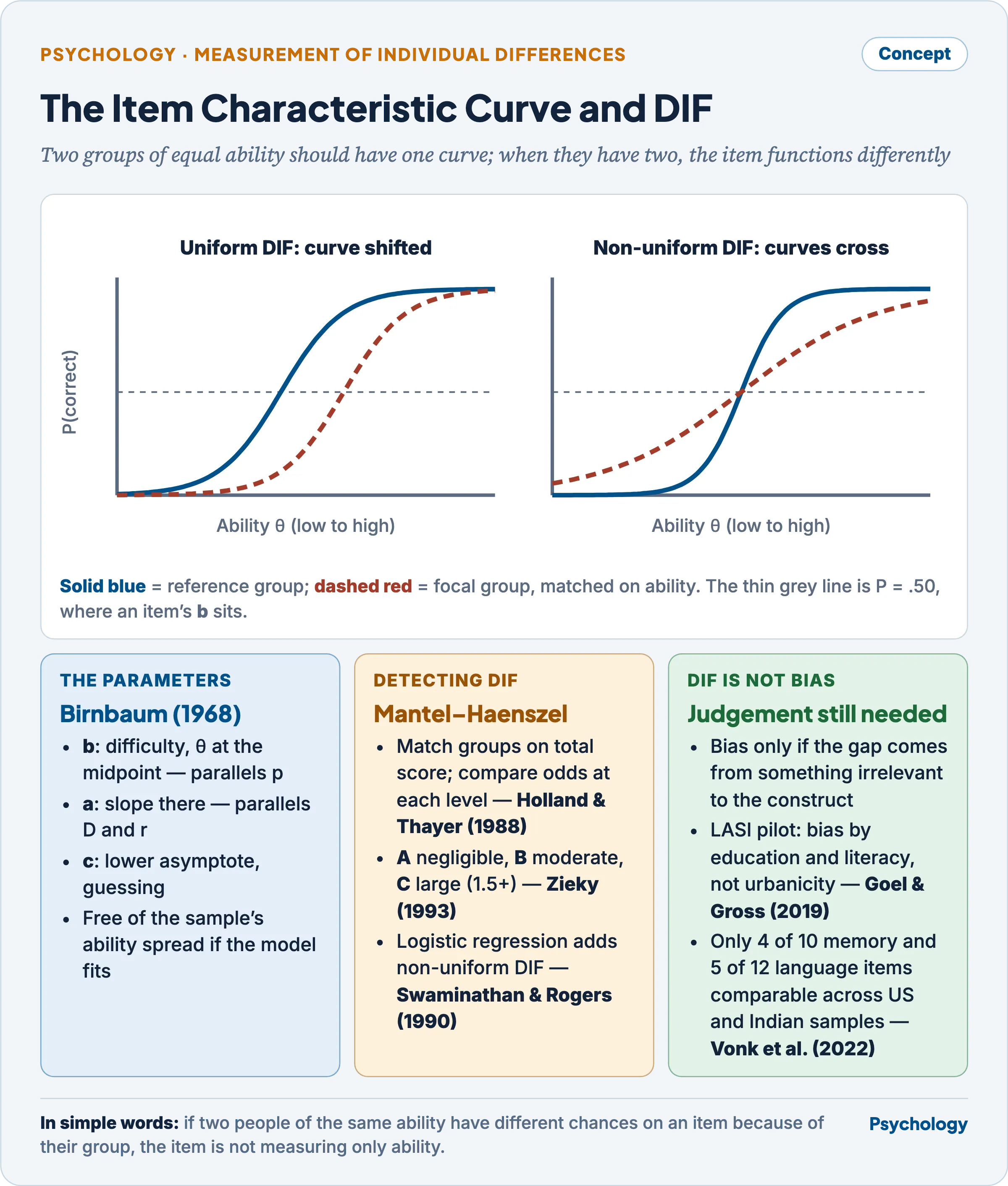
Equal ability, unequal chance: the gap between the two curves at any one ability level is the DIF.
Exploratory, confirmatory and integrated factor analysis in test construction
- Factor analysis tests dimensionality — whether the items measure as many attributes as intended. Extraction and rotation are in Factor Analysis and Multivariate Techniques (Paper I).
- Items need their own correlations: Ferguson (1941) showed that phi coefficients among same-content items of differing difficulty produce spurious difficulty factors, and Wherry and Gaylord (1944) recommended tetrachoric correlations — polychoric for rating items.
- Exploratory factor analysis (EFA) suits an unknown structure: a new construct or item pool, or an imported test whose structure in a new culture is in doubt.
- Good practice — common factors, oblique rotation, parallel analysis (Horn, 1965) rather than eigenvalues above one (Kaiser, 1960) — was widely ignored in published research (Fabrigar, Wegener, MacCallum and Strahan, 1999).
- Confirmatory factor analysis (CFA) (Jöreskog, 1969) suits a structure fixed by theory or prior work: adapting an established test, comparing rival models, or testing measurement invariance across languages.
- Conventional fit cut-offs: CFI at least .95, RMSEA at most .06, SRMR at most .08 (Hu and Bentler, 1999).
- The integrated approach uses both, in order, on separate data.
- Split the sample: EFA on one half, its solution tested by CFA on the other. Gerbing and Hamilton (1996) found by simulation that EFA recovered the true model well except in small samples with highly correlated factors.
- Anderson and Gerbing (1988), in the two-step approach, test and respecify the measurement model by CFA before estimating structural relations.
- Exploratory structural equation modelling (ESEM) (Asparouhov and Muthén, 2009) keeps EFA’s cross-loadings inside a confirmatory model, because CFA’s zero cross-loadings misfit real items and inflate factor correlations.
- Marsh and colleagues (2010) found item-level CFA rejected the NEO Five-Factor Inventory’s structure in 3,390 respondents, while ESEM fitted better with less correlated factors.
| Dimension | EFA | CFA | Integrated (EFA → CFA, or ESEM) |
|---|---|---|---|
| Starting point | No defensible prior structure | Structure specified in advance | Structure known in outline; cross-loadings expected |
| Can it fail? | No: always returns a solution | Yes: the model can be rejected | Yes, at the confirmatory stage |
| Use in test construction | Screening a new pool | Adapting a test; invariance across groups | New test with a predictive blueprint; personality items |
| Main risk | Subjective retention and naming | Over-strict model; modifying until it fits | One sample used for both stages |
- The cardinal error is EFA and CFA on the same data; and a CFA modified until it fits has become an EFA.
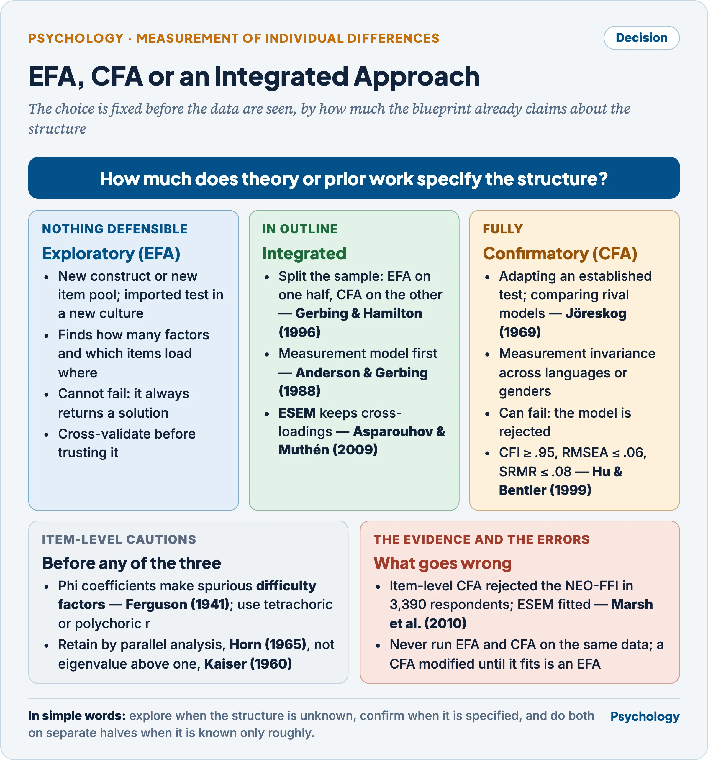
The choice is made before the data are seen — by how much the blueprint already claims about the structure.
Criticisms and limitations
- Sample dependence — p, D and r-pbis shift with the try-out group’s ability spread.
- Chance capitalisation — choosing the best-looking items from a few hundred testees exploits sampling error (Cureton, 1950).
- Circular internal criteria — item–total statistics measure agreement with other items, not validity; DIF matching on total score inherits this.
- Homogeneity bought with breadth — the attenuation paradox (Loevinger, 1954).
- Blindness to consistent irrelevance — statistics assume the pool samples the construct; blueprint and expert review do what no index can.
- Conventions mistaken for laws — the 27 per cent rule rests on normality (Cureton, 1957); D bands and fit cut-offs are rules of thumb a wrong model can meet.
- Speed and translation make not-reached and non-equivalent items look hard or biased.
Indian context
- National Achievement Survey (Ministry of Education; NCERT) — operationalises common-scale measurement: items calibrated together let booklets, languages and years share one metric, if each item works the same everywhere.
- In the 2017 survey, four-option items written in English were translated and field-tested in 20 languages; classical test theory served district results and item response theory the national scale.
- The 2018 Class X round chose the two-parameter over the Rasch model because item discriminations were not comparable, and dropped any item misfitting in a state from that state’s scoring alone.
- PARAKH (Ministry of Education, under NCERT; set up 8 February 2023 following NEP 2020) — operationalises translation equivalence across its languages.
- Its PARAKH Rashtriya Sarvekshan, successor to the survey, tested Grades 3, 6 and 9 on 4 December 2024 in 23 languages: over 21.15 lakh students in 781 districts.
- Longitudinal Ageing Study in India (LASI; Ministry of Health and Family Welfare; Wave 1 2017–18, 72,250 adults aged 45 and over and their spouses) — operationalises fairness across literacy, so that little schooling is not misread as cognitive decline.
- Goel and Gross (2019) found the cognitive items of its 2010 pilot biased by education and literacy but not urbanicity, animal-fluency items among those flagged.
- Vonk and colleagues (2022), harmonising a US sample (3,496) with the LASI dementia sub-study (3,152; 12 Indian languages), found only 4 of 10 memory and 5 of 12 language items comparable.
- Gross and colleagues (2020) confirmed that sub-study battery’s structure by CFA and found it invariant across its language versions.
- Chauhan, Chauhan, Vaza and Chauhan (2023) analysed 200 four-option MCQs taken by 400 medical graduates in Gujarat (KR-20 .91): mean p 57.75 per cent, mean D 0.44, and items with three functioning distractors discriminated best.
Previous Year Questions
- 2019How can one make a decision of using exploratory factor analysis or confirmatory factor analysis or an integrated approach while constructing a psychological test?
- 2017What is the role of item validation in psychometric scaling? Briefly describe the steps involved.
- 2014What is the purpose of item analysis? How would you carry it out for a test of aptitude?