Factor Analysis and Multivariate Techniques in Psychology

Application of statistical technique (factor analysis).

Official Syllabus: Paper I · Unit 3 Research Methods

“The principal concern of factor analysis is the resolution of a set of variables linearly in terms of a small number of categories or factors.”

— Harman (1967)

Factor analysis exists because psychology measures many things that turn out to be measuring fewer. Spearman (1904) invented it on exactly that observation: every test of mental ability correlated positively with every other, and he proposed that a single general factor plus a factor specific to each test would account for the whole pattern. The technique has since become the standard instrument for asking what structure lies beneath a correlation matrix, and the standard instrument for abusing that question.

When factor analysis becomes necessary

The technique is called for under conditions that can be stated precisely, and it is not a general-purpose tool.

• A large number of intercorrelated variables, and a question about their structure. Fifty items, twenty tests or thirty ratings whose correlations are substantial, and the investigator wants to know how many distinct things are being measured. A correlation matrix of fifty variables has 1,225 coefficients, which no one can read.
• Construct validation. A test claims to measure four dimensions; factor analysis asks whether four dimensions are what the item responses actually display, and whether the items group as the manual says.
• Test and scale construction. At the item-pool stage it identifies which items belong together, which load on no factor and should be discarded, and which load on several and are therefore ambiguous. It also establishes the dimensionality that item response theory requires before it can be applied.
• Testing a theory about latent structure. Whether ability is one thing or several, and whether personality has five dimensions or three, are factor-analytic questions and were settled — to the extent they are settled — factor-analytically.
• Data reduction before another analysis. Where predictors are heavily intercorrelated, factor scores replace them in a regression and remove the multicollinearity.
• Detecting method variance. Where items sharing a response format load together irrespective of content, the shared method is operating as a factor.

It is not called for when the variables are few or essentially uncorrelated, when the aim is prediction rather than structure, or when the sample is too small — a conventional minimum is five to ten cases per variable, and the stability of a solution depends more on sample size and on the size of the loadings than on any rule of thumb.

The procedure

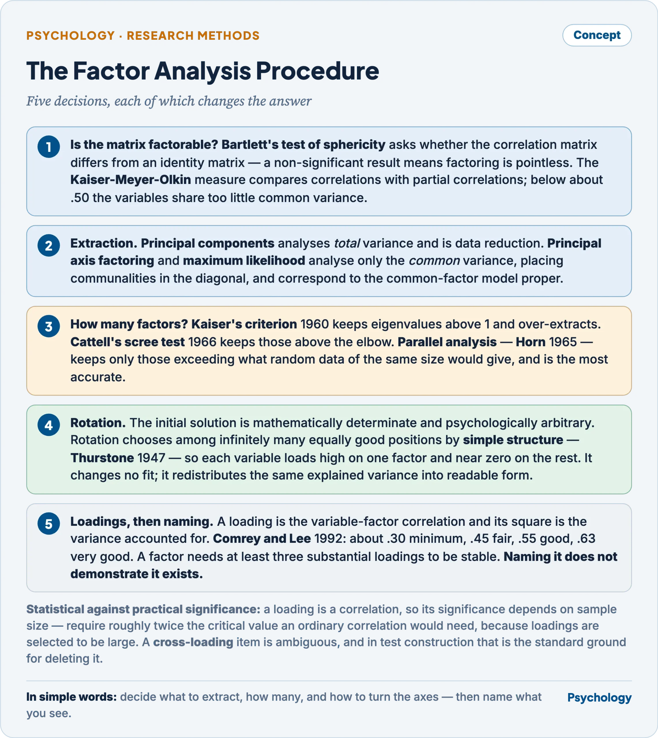
Each decision changes the answer the analysis returns.

Checking that the matrix is factorable

Before extraction, two checks establish whether there is any common variance to analyse. Bartlett’s test of sphericity asks whether the correlation matrix differs from an identity matrix; a non-significant result means the variables are unrelated and factoring is pointless. The Kaiser-Meyer-Olkin measure of sampling adequacy compares the magnitudes of correlations with those of partial correlations, and values below about .50 indicate the variables do not share enough common variance.

Extraction

• Principal components analysis transforms the variables into uncorrelated components accounting for total variance, and is strictly a data-reduction method rather than a model of latent causes.
• Principal axis factoring and maximum likelihood extraction analyse only the common variance shared among variables, placing communalities rather than unities in the diagonal, and correspond to the common-factor model proper. Maximum likelihood also supplies a significance test for the number of factors.
• The communality of a variable is the proportion of its variance accounted for by the common factors; the remainder is its uniqueness, comprising specific variance and error.
• An eigenvalue is the amount of variance a factor accounts for, expressed in units of a single variable’s variance.

Deciding how many factors

• Kaiser’s criterion (1960) retains factors with eigenvalues above 1, on the ground that a factor should account for at least as much variance as a single variable. It systematically over-extracts and should not be used alone.
• Cattell’s scree test (1966) plots eigenvalues in order and retains those above the elbow where the curve flattens into scree.
• Parallel analysis, from Horn (1965), retains only factors whose eigenvalues exceed those obtained from random data of the same size, and is the most accurate of the three.
• Interpretability and theory decide between close alternatives. A statistically defensible factor nobody can name is usually an artefact.

Rotation

The initial solution is mathematically determinate and psychologically arbitrary: infinitely many positions of the axes fit the data equally well. Rotation chooses among them by a criterion of interpretability, which Thurstone (1947) formalised as simple structure — each variable should load highly on one factor and near zero on the others, and each factor should have several variables loading near zero on it. Rotation changes no fit; it redistributes the same explained variance into a form that can be read.

• Orthogonal rotation keeps the factors uncorrelated.
  • Varimax, from Kaiser (1958), maximises the variance of squared loadings within each factor, simplifying the columns so that each factor has a few high and many near-zero loadings. It is the most widely used rotation.
  • Quartimax simplifies the rows, so that each variable loads on as few factors as possible. It tends to produce a large general factor on which everything loads.
  • Equamax is a compromise between the two.
• Oblique rotation allows the factors to correlate.
  • Direct oblimin, promax and quartimin are the standard methods. They produce three matrices rather than one: a pattern matrix of unique contributions, a structure matrix of variable-factor correlations, and a factor correlation matrix.
  • Oblique solutions also permit higher-order factors to be extracted from the correlations among the first-order factors, which is how a general factor is recovered from correlated primary abilities.
• Choosing between them. Orthogonal rotation gives simpler interpretation and uncorrelated factor scores, and is defensible when the constructs are theoretically independent — the position associated with Guilford. Oblique rotation is the more realistic choice in psychology, where traits and abilities almost always correlate, and is the position associated with Thurstone and Cattell. The practical rule is to rotate obliquely first: if the factor correlations prove negligible, the orthogonal solution is justified and can be adopted; if they are substantial, forcing orthogonality distorts the structure.

Factor loadings and their significance

A factor loading is the correlation between a variable and a factor in an orthogonal solution, and its square is the proportion of that variable’s variance accounted for by that factor.

• Statistical significance depends on sample size, since a loading is a correlation. The conventional guidance is to require roughly twice the critical value an ordinary correlation would need at that sample size, because the loadings are selected to be large. In a sample of 100 this places the threshold near .50, while in a sample of 300 a loading of about .30 suffices.
• Practical significance is judged by magnitude, and the conventional bands are those of Comrey and Lee (1992): around .30 is the minimum worth interpreting, .45 is fair, .55 good and .63 or above very good. The reasoning is the squared loading — a loading of .55 means the factor accounts for about 30 per cent of that variable’s variance.
• Cross-loading — a variable loading above the threshold on two or more factors — makes that variable ambiguous, and in test construction it is the standard ground for deleting an item.
• A factor should carry at least three substantial loadings to be stable and interpretable; a factor defined by two variables is usually a doublet rather than a dimension.

Naming and interpretation

The factor is named from what its highly loading variables have in common, and this is the step where factor analysis is most often over-read. Naming a factor does not demonstrate that it exists. The label is an inference from a pattern of correlations, it carries all the investigator’s prior expectations, and the same matrix has been named differently by different investigators. The honest treatment is to regard the name as a hypothesis the rest of the research programme must support.

Exploratory and confirmatory factor analysis

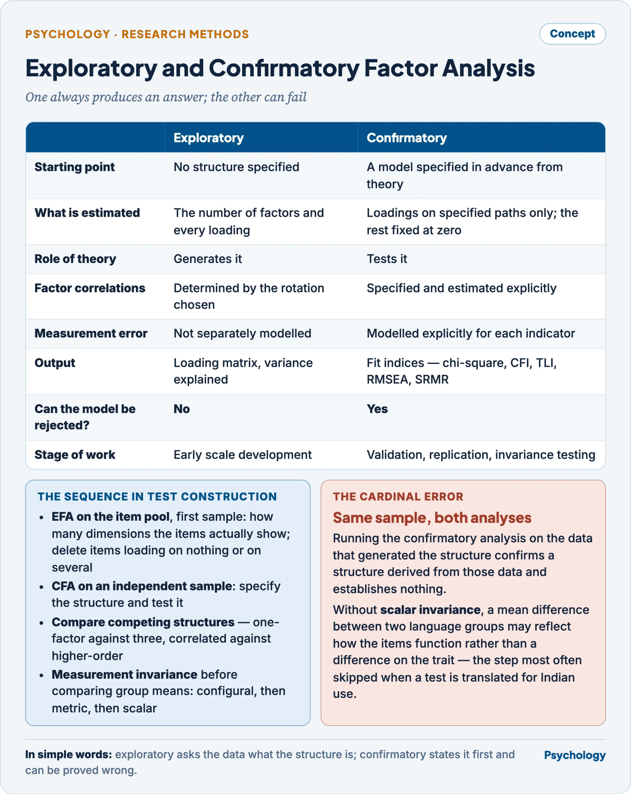
One always produces an answer; the other can fail.

The decisive difference is that an exploratory analysis always produces an answer and a confirmatory one can fail. Exploratory factor analysis asks the data what the structure is; confirmatory factor analysis states the structure first and reports how badly the data depart from it, which makes it a genuine test.

Their significance in test construction

The two belong at different stages of one sequence, and the sequence is what makes a test defensible.

• Exploratory analysis on the item pool, in a first sample: it reveals how many dimensions the items actually display, which may not be the number intended; it identifies items that load on nothing, which measure something else or nothing; and it identifies cross-loading items, which are ambiguous. Items are deleted and subscales formed on this basis.
• Confirmatory analysis on an independent sample: the structure found is specified as a model and tested. Fit indices report whether the hypothesised structure reproduces the observed covariances, and modification indices show where it fails.
• Competing structures are compared — a one-factor against a three-factor model, a correlated-factors against a higher-order model — which exploratory analysis cannot do, since it cannot reject anything.
• Measurement invariance is tested across groups before their scores are compared: configural invariance establishes the same pattern, metric invariance the same loadings, scalar invariance the same intercepts. Without scalar invariance, a difference in mean scores between two language groups or two regions may reflect how the items function rather than a difference on the trait. This is the technical basis of fairness in testing and the step most often skipped when a test is translated for Indian use.
• The cardinal error is running the exploratory and confirmatory analyses on the same data, which confirms a structure derived from those data and establishes nothing.

Multivariate techniques in psychological research

Multivariate techniques handle several variables simultaneously rather than one outcome at a time, and they divide by whether a dependent variable is identified.

Dependence techniques, where one or more outcomes are predicted or explained:

• Multiple regression — one continuous outcome from several predictors. Prediction, control of confounds, relative importance.
• Analysis of covariance — a treatment effect on one outcome with a covariate’s variance removed, raising precision in quasi-experimental comparisons.
• MANOVA — several correlated outcomes tested at once. It controls the familywise error rate that separate ANOVAs would inflate, and it can detect an effect on a combination of outcomes that no single outcome shows. Used where a treatment is expected to affect a syndrome rather than one symptom.
• MANCOVA — the same, with covariates removed.
• Discriminant function analysis — predicts group membership from continuous predictors, and identifies which predictors separate the groups. Used in selection, in differential diagnosis, and in classifying applicants.
• Logistic regression — a categorical outcome from any mixture of predictors, giving odds ratios; it has largely displaced discriminant analysis because it assumes less.
• Canonical correlation — the relation between one set of variables and another set, such as a battery of ability tests against a battery of job-performance measures.
• Path analysis and structural equation modelling — a specified network of directed relations among variables, with SEM combining a measurement model of latent variables with a structural model of relations among them, and correcting for measurement error in doing so.
• Multilevel modelling — data with a nested structure, such as pupils within classes within schools, where observations are not independent.

Interdependence techniques, where no variable is singled out as an outcome:

• Factor analysis and principal components — the latent dimensions underlying a set of variables.
• Cluster analysis — groups cases rather than variables by their similarity, producing typologies of patients, consumers or organisations.
• Multidimensional scaling — recovers a spatial map from judgements of similarity, so that the dimensions people actually use to compare occupations, colours or political parties can be read off without being specified in advance.

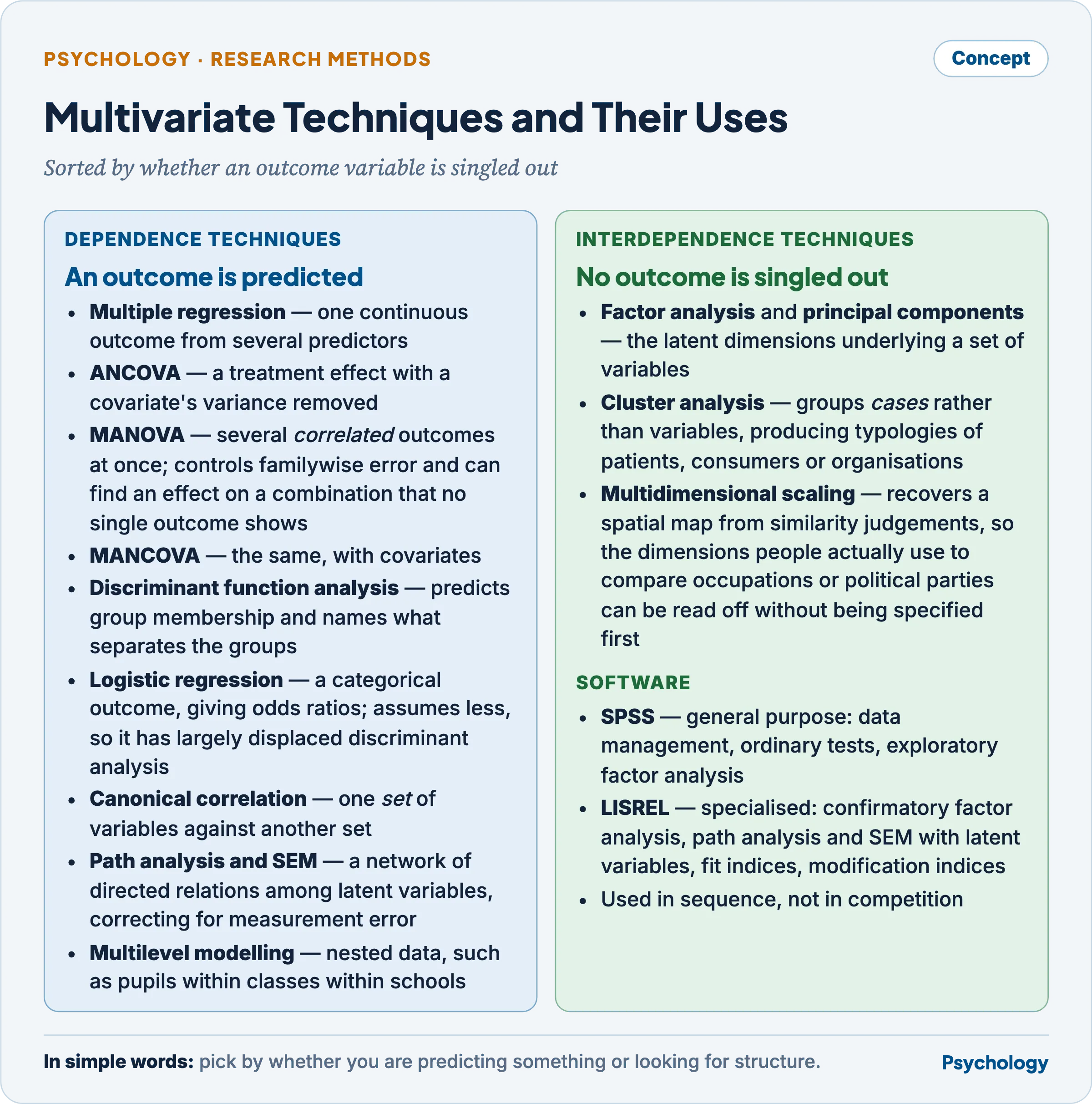
Sorted by whether an outcome variable is singled out.

Statistical software: LISREL and SPSS

The two are not competitors so much as instruments of different scope, and the comparison turns on what each can model.

• SPSS is a general-purpose package: data management, descriptive statistics, t-tests, ANOVA and MANOVA, correlation and regression, non-parametric tests, reliability analysis and exploratory factor analysis, driven through menus as well as syntax. Its breadth and its menu interface are why it is the first package most researchers learn.
• LISREL, from Jöreskog and Sörbom, is a specialised program for the analysis of covariance structures — confirmatory factor analysis, path analysis and full structural equation modelling with latent variables. It takes a covariance or correlation matrix as its input, estimates the measurement model and the structural model simultaneously, corrects relations among constructs for measurement error in the indicators, and reports goodness-of-fit indices and modification indices.
• What LISREL does that base SPSS cannot. Specify and test a hypothesised factor structure; reject a model; model latent variables with explicit error terms; estimate correlated errors; test measurement invariance across groups; and fit a system of simultaneous equations. SPSS’s exploratory factor analysis produces a solution whatever the data, supplies no fit indices and models no measurement error.
• What SPSS does that LISREL does not. Routine data preparation, recoding and merging; descriptive and exploratory work; the whole range of ordinary significance tests; and the exploratory factor analysis that normally has to precede a confirmatory model.
• In practice they are used in sequence — SPSS to prepare data and run the exploratory analysis, LISREL to test the resulting model on a second sample. The specialised role has since been taken up by AMOS, Mplus and the open-source alternatives, which do the same covariance-structure work with easier interfaces, so LISREL’s distinction today is historical as much as functional.

Criticisms and limitations

• Factor analysis cannot discover causes. It describes the correlational structure of a set of measures. That a general factor can be extracted shows that the measures intercorrelate, not that a single underlying entity exists — the standard objection to the reification of g, and the reason competing factor models of intelligence have coexisted for a century on the same data.
• The solution is not unique. Different extraction methods, different numbers of factors retained and different rotations yield different and equally well-fitting structures, each of which can be named plausibly. The investigator’s choices do much of the work attributed to the data.
• Garbage in, structure out. Factor analysis finds dimensions in whatever is entered, so the factors cannot be richer than the item pool. A personality inventory missing an entire domain will return a tidy structure with that domain absent.
• Sample size and stability. Solutions from small samples do not replicate, and the literature contains many structures established once and never since.
• Confirmatory fit indices are conventions. The cut-offs in general use are rules of thumb from simulation studies, a model can fit well and be substantively wrong, and modification indices invite the respecification of a model until it fits — which turns a confirmatory analysis back into an exploratory one while retaining the language of testing.
• Multivariate techniques are frequently applied to designs that cannot support them. Structural equation modelling in particular carries causal diagrams and causal vocabulary while resting, in most applications, on cross-sectional correlational data; a fitting model is one of many that fit equally, and fit is not evidence of the direction of the arrows.