

Question: “Geomorphic scale is a significant parameter in the interpretation of landform development and landform characteristics of geomorphic systems.” Discuss.
Introduction: Time and Space as Active Variables
The statement builds on the celebrated Schumm & Lichty (1965) argument in “Time, Space and Causality in Geomorphology”: scale is not a neutral frame — it is an active parameter that determines which variables are dependent, which independent, and which irrelevant in any interpretation. A process that is cause at the instantaneous scale becomes effect at the graded scale, and diminishes to background noise at the cyclic scale. Interpreting a landform assemblage without fixing temporal and spatial scale is therefore meaningless — the same feature (a knickpoint, a river terrace, an erosion surface) is read differently at different resolutions. The statement is true and pivotal: geomorphic scale dictates model choice (Davisian cyclic vs Hackian dynamic equilibrium), variable selection, and the very meaning of the “system” being studied.
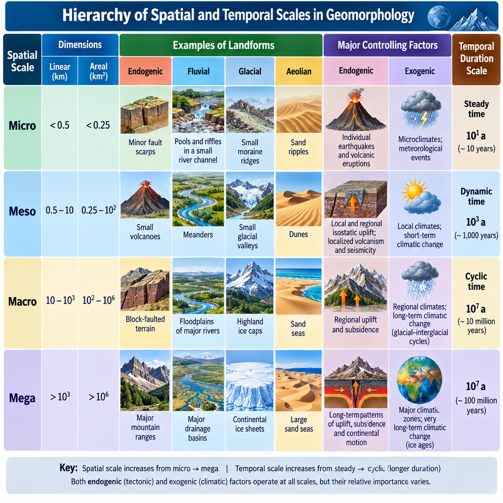
1. The Two Scales: Temporal and Spatial
- Temporal scale — three canonical divisions after Schumm & Lichty:
- Cyclic time (10⁵–10⁸ yr): the span of a Davisian cycle — landscapes conceived as evolving sequences; historical/denudational interpretation dominates.
- Graded time (10³–10⁵ yr): the span over which short-term fluctuations (individual floods, storms) average out; the landform attains dynamic equilibrium about a progressively changing mean (graded stream — Mackin).
- Steady time (10⁰–10² yr): the span over which averages are static; the system is in constant equilibrium, and instantaneous inputs–outputs (e.g., a flood year) are the relevant measures.
- Spatial scale — the areal/geometric extent of the system: from the first-order (the world/landmass) to second/third order (regions, drainage basins), fourth order (valley reaches, slope units), and fifth order (individual landforms — a dune, a channel bar, a soil pedon).
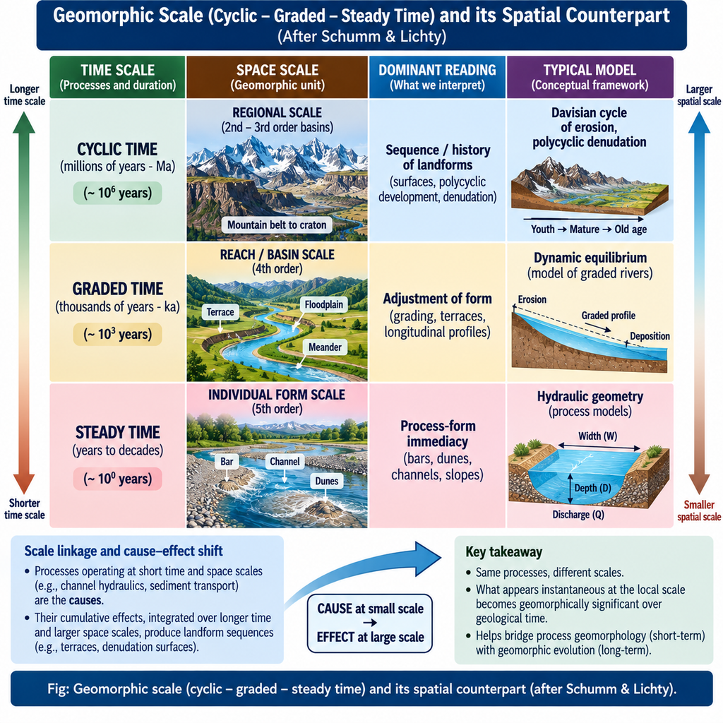
- Temporal–spatial coupling (Schumm & Lichty’s profound insight): cyclic time ↔ second/third-order (regional) landforms; graded time ↔ fourth-order (reach/valley) landforms; steady time ↔ fifth-order (individual form) landforms. Each analysis must pair its time scale with its matching spatial scale.
2. How Scale Changes the Interpretation (the “Scale Table”)
| Time scale | Space scale | What is “cause” | What is “effect” | Typical model |
|---|---|---|---|---|
| Cyclic (Ma) | Regional/provincial (2nd–3rd order) | Uplift, eustasy, climate state, denudation budget | Erosion surfaces, polycyclic assemblages, peneplain remnants | Davisian sequence; denudation chronology |
| Graded (ka–Ma) | Basin/reach (4th order) | Base level, discharge regime, sediment supply | Channel pattern, terrace formation, valley gradient | Graded profile; dynamic equilibrium (Hack) |
| Steady (yr–decade) | Individual form (5th order) | Discharge, sediment input, roughness | Cross-section shape, bar/dune dimensions, bedform migration | Hydraulic geometry; bedform theory |
- Read in reverse, the same landform is interpreted differently by the scale lens applied: e.g., a Himalayan river terrace is (steady) a flood-erosional coupon, (graded) a response to monsoon sediment regime, (cyclic) a relict of Pleistocene glacio-eustasy or a signal of ongoing Himalayan uplift — the parameter of scale decides the reading.
3. Scale Determines the Model and the Paradigm
- Large geomorphic scale (cyclic, regional) → time-dependent (historical) approaches: Davis’s cycle, denudation chronology, palaeogeomorphology. Interprets landscapes as sequences through time.
- Small geomorphic scale (steady, local) → time-independent (functional/process) approaches: Hack’s dynamic equilibrium, hydraulic geometry, process-form studies. Interprets landscape as adjusted form to present processes.
- The scale trap: applying cyclic-time concepts to a steady-time observation (e.g., treating a present-day gully as evidence of a “young” landscape) or the reverse (ignoring inherited surfaces because today’s processes are active) produces fallacious interpretation. The discipline’s great paradigm split — historical vs process geomorphology — is fundamentally a scale dispute.
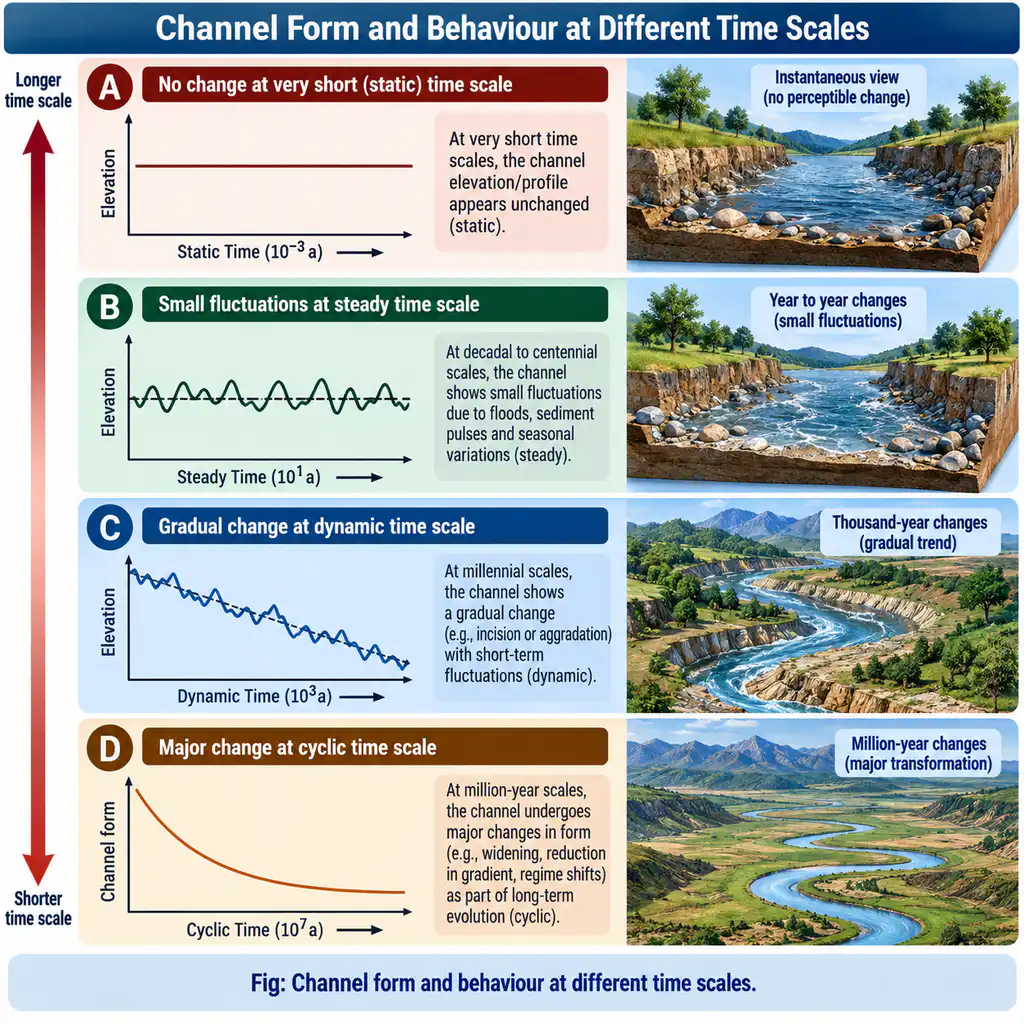
4. Evidence and Applications from the Field
- Indian examples of scale dependency:
- Chotanagpur polycyclic surfaces (cyclic scale): Netarhat ~1,065 m (Jurassic), Ranchi ~650–700 m (mid-Tertiary), Chaibasa 150–300 m (late Pliocene–Pleistocene) — a regional-cyclic reading; at the steady scale the same tract shows modern incision of the Subarnarekha (Hundrughagh falls 74 m) — present-day process.
- Kosi megafan: cyclic scale — a late-Quaternary fan system recording Himalayan uplift and sediment pulsing; graded scale — its ~133 km westward avulsion between 1736–1968 shows channel-pattern adjustment to sediment load; steady scale — year-to-year braid-planform shifts at 150–170 m/yr thread migration.
- South Lhonak/GLOF (Sikkim 2023): steady-time (decades) observation — lake expanded 12-fold (0.11→1.4 km², 1962–2023) and glacier thinning accelerated (–0.19→ –0.87 m/yr) — predates/cascades into a graded-time system change (moraine instability); interpretation is scale-jumping — the classic proof that interpretation requires scale awareness.
- Coastal: a beach is a steady-time sediment cell; a barrier-lagoon system a graded-time response; a sequence of raised beaches/stranded dune ridges a cyclic-time (sea-level oscillational) record (INCOIS projects 0.62–0.87 m relative sea-level rise by 2100 for India’s coast — a graded-to-cyclic future signal).
- Dating techniques (see also Q29, Q31) make scale operational: ¹⁰Be exposure dating resolves steady/grade time (10³–10⁵ yr) horizons; stratigraphy resolves cyclic time — hence the recent turn to scale-resolved chronology in Himalayan denudation studies (Kosi catchment denudation 0.12 mm/yr at 4.4 Ma → 4.4 mm/yr in the Holocene).
5. Scale and Geomorphic Systems: The Systems Connection
- In systems geomorphology, scale fixes the boundary conditions of the system: an open system at one scale is a closed store within a larger system, or a single “input” to a smaller one. Feedback loops that are internal at one scale become external forcing at another — so the system characteristics (self-regulation vs transience, equilibrium vs disequilibrium) are scale-laden.
- Connectivity and hierarchy: modern geomorphology couples hierarchical (nested) scaling theory with connectivity by noting that changes at fifth-order (bar, riffle) aggregate to fourth-order (reach) adjustments, which cumulate to third-order (basin) responses — but with memory/filters along the cascade (sediment pulsing, thresholds), so that the pattern is neither purely bottom-up nor top-down. Scale is thus an emergent property of the coupled system, not merely a viewing lens.
6. Conclusion
The statement is profoundly correct. Geomorphic scale — the pair of temporal and spatial resolutions at which an investigation is framed — is not a passive margin note but an active, controlling parameter of interpretation: it decides which variables are causes and which are effects (Schumm & Lichty), whether a landform is read as a Davisian sequence or a Hackian equilibrium, which data are relevant (steady gauge records vs stratigraphic columns vs cosmogenic rates), and which geomorphic system’s boundaries and feedbacks define the object of study. The practical lesson for the geomorphologist is scale discipline: always pair cyclic time with regional space, graded time with reach scale, steady time with individual forms — and treat “significance” as scale-bound. This is precisely why the same Indian landscape — Chotanagpur surfaces, Kosi fan, Sikkim lakes, Indian coasts — yields different truths at different scales, and why modern geomorphology is a multi-scale, scale-aware science.