

Question: Explain the major techniques used in denudation chronology.
Introduction: The Multi-Tiered Methodological Toolkit
Denudation chronology reconstructs the historical biography of a landscape — establishing when, at what rate, and through what physical sequence subaerial erosion lowered the land surface through geological time. Because landscapes are complex, polycyclic palimpsests where fragments of ancient base-levelled surfaces coexist alongside actively incising gorges, no single method suffices.
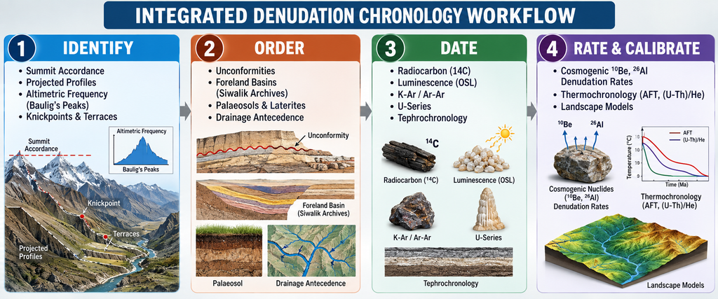
Modern denudation chronology operates across an integrated, four-tier methodological workflow:
- Tier 1: Morphological & Morphometric Identification: Mapping and isolating relict planation fragments and breaks of slope.
- Tier 2: Stratigraphic & Sedimentary Correlation: Ordering the relative sequence of erosional and depositional events.
- Tier 3: Geochronometric & Radiometric Dating: Calibrating absolute calendar ages for surfaces, fills, and capping rocks.
- Tier 4: Cosmogenic Radionuclide & Thermochronological Rating: Quantifying catchment-wide denudation rates (in mm/year) and deep-crustal exhumation trajectories.
1. Tier 1: Morphological & Morphometric Identification Techniques
These techniques detect and trace the physical fragments of former erosion surfaces before chemical or isotopic dating is attempted:
A. Summit Accordance & Serial Profile Analysis
- Summit Accordance: By plotting the peak elevations of residual hills across a region, geomorphologists identify concordant heights that signify a dissected, belevelled paleosurface.
- Serial Profile Techniques:
- Superimposed Profiles: Multiple parallel topographic profiles are plotted together on a single cross-section. The lowest envelope reveals continuous valley flats, while the upper envelope traces accordant summit levels.
- Projected Profiles: Intervening valleys are omitted, projecting only the prominent ridgelines onto a single vertical plane to highlight planar upland benches.
- Composite Profiles: Represents the highest surface elevations across a grid, revealing ancient surfaces bevelled across diverse lithologies.
B. Baulig’s Altimetric Frequency Analysis (1950s)
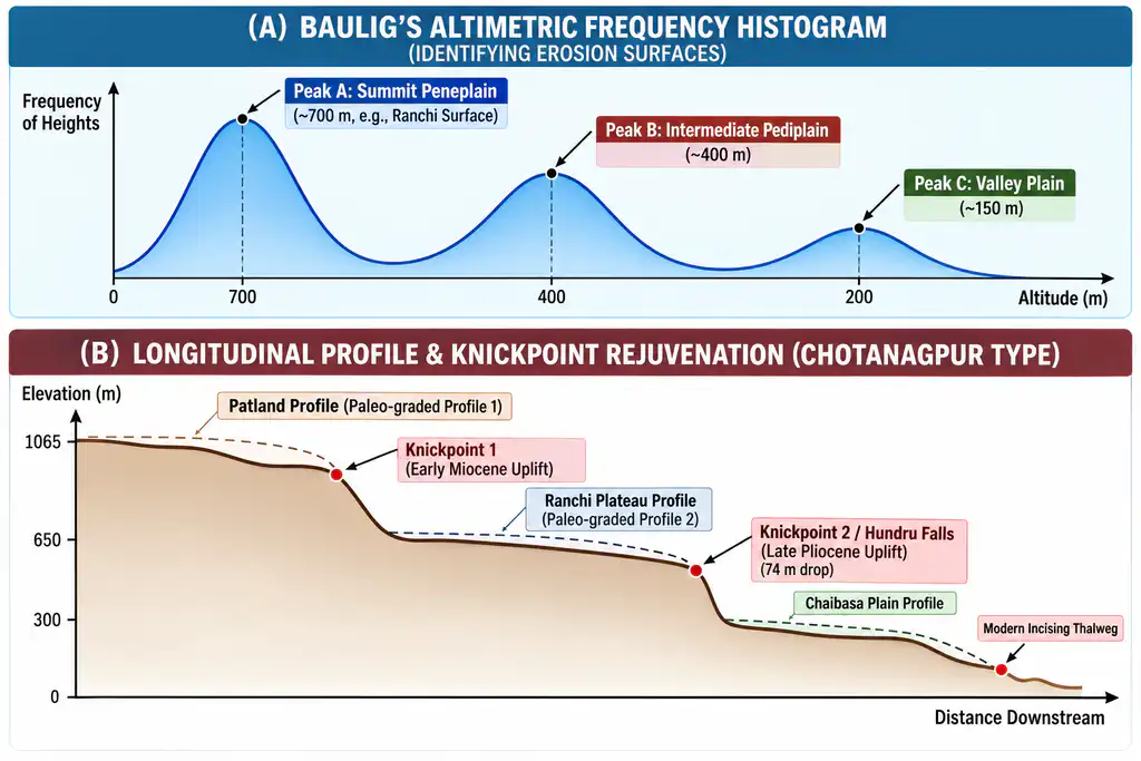
- Pioneered by Henri Baulig, this statistical morphometric technique tabulates the frequency of spot heights, summit contours, and bench elevations within a drainage basin.
- When plotted as a frequency histogram or curve, statistically significant modal peaks correspond directly to former planation levels (erosion surfaces).
- Indian Application: In the Belan Basin (U.P.), Savindra Singh and R. Srivastava (1976) plotted altimetric frequency histograms, revealing four distinct modal peaks corresponding to the Kaimur Surface (427 m), Panna Surface (305 to 366 m), Rewa Surface (240 m), and Trans-Yamuna-Ganga Surface (150 m).
C. Hypsometric Analysis (Strahler, 1952)
- Plots relative height against relative area within a drainage basin.
- The Hypsometric Integral (HI) diagnoses the evolutionary maturity of the landscape:
- Youthful / Actively Uplifting Basin (HI greater than 0.60): Convex curve with high mass remaining; deep V-shaped valleys.
- Mature Equilibrium Basin (HI between 0.35 and 0.60): S-shaped profile with balanced slope distribution.
- Monocyclic Peneplained / Old-Age Basin (HI less than 0.35): Deeply concave curve representing extensive planar reduction.
D. Longitudinal River Profiles & Knickpoint Analysis
- A fully graded river exhibits a smooth, concave-upward longitudinal profile. Tectonic rejuvenation, base-level drop, or river capture introduces abrupt convex breaks of slope called knickpoints (nickpoints).
- Knickpoints migrate headward (retrogressive erosion), separating the relict, older valley upstream from the incising, juvenile valley downstream.
- Hack’s Stream-Length Gradient Index (SL Index):SL Index = (Channel Slope) × (Total Channel Length) = (ΔH / ΔL) × L
(Where ΔH / ΔL is local channel gradient, and L is channel length from drainage divide). Abnormally high SL anomalies isolate active tectonic knickzones and quantify rejuvenation pulses (e.g., Narmada and Chambal gorges).
E. River Terrace Staircases
- Stepped sequences of strath (bedrock-cut) and fill (alluvial accumulation) terraces record cyclic alternations between lateral planation and vertical incision driven by glacio-eustatic or tectonic forcing.
2. Tier 2: Stratigraphic & Sedimentary Correlation Techniques
Stratigraphic relationships establish the relative temporal sequence and environmental conditions:
- Unconformity Mapping: An unconformity represents a preserved fossil erosion surface dividing older, folded or crystalline basement rocks from younger, flat-lying sedimentary strata. It proves that an ancient planation cycle operated prior to burial (e.g., the Great Eparchaean Unconformity of Peninsular India).
- Correlated Foreland Basin Archives: As highlands are denuded, the eroded detritus is deposited in adjacent foreland basins, preserving an inverted chronological record:
- The Siwalik Foreland Record: The 6,000-metre-thick Siwalik succession in northern India documents the unroofing history of the Himalayas from the middle Miocene to early Pleistocene. Coarsening-upward facies (from fine mudstones to massive boulder conglomerates of the Upper Siwaliks) calibrate specific tectonic pulses and unroofing of Lesser and Greater Himalayan crystalline complexes.
- Palaeosols & Weathering Duricrusts: Capping sheets of laterite, bauxite, silcrete, or calcrete signify prolonged subaerial chemical weathering under tectonic quiescence. The bauxitic laterite cappings of the Netarhat Patlands (Jharkhand) and Panchpatmali (Odisha) serve as regional chronostratigraphic markers.
- Drainage Discordance (Antecedence & Superimposition):
- Antecedent Rivers: Trans-Himalayan gorges of the Indus, Sutlej, and Brahmaputra prove these rivers predate Himalayan orogeny, providing a minimum chronological boundary.
- Superimposed Rivers: The Damodar and Subarnarekha cut across ancient metamorphic structures of Chotanagpur, demonstrating former burial beneath now-stripped cover rocks.
3. Tier 3 & 4: Geochronometric & Quantitative Dating Techniques
Modern denudation chronology pairs classical relative ordering with high-precision absolute chronometry and low-temperature thermochronology:
| Technique | Physical System & Material | Effective Temporal Range | Diagnostic Geomorphic Application |
|---|---|---|---|
| Radiocarbon (14C) | Organic carbon, charcoal, peat, shell | 0 to 50,000 years | Dating Holocene river terraces, alluvial fills, and paleoseismic fault scarps. |
| Optically Stimulated Luminescence (OSL / IRSL) | Quartz and K-feldspar sand grains | 100 to 300,000 years | Dating the burial time of alluvial terraces, sand dunes, and paleochannels. |
| Argon-Argon (40Ar/39Ar) / K-Ar | Volcanic minerals, basalt flows, ash | Greater than 100,000 years (up to billions of years) | Dating basalt sheets capping planation surfaces (e.g., Deccan Traps, approx. 65 million years old, bracketing Gondwana surfaces). |
| Uranium-Series (230Th/234U) | Cave speleothems, corals, travertine | 1,000 to 500,000 years | Calibrating marine terraces, coastal planation benches, and karst evolution. |
| In-situ Cosmogenic Radionuclides (10Be, 26Al, 36Cl) | Quartz in river sand and bedrock surfaces | 1,000 to 5 million years | Catchment-wide denudation rates (in mm/year) and exposure dating of bedrock scarps. |
| Low-Temperature Thermochronology: Apatite Fission-Track (AFT) | Apatite crystals in crystalline rocks | 1 to 100 million years | Tracks cooling through approx. 110°C (approx. 3 to 4 km crustal depth), yielding long-term exhumation rates. |
| Low-Temperature Thermochronology: (U-Th)/He (AHe) | Apatite and zircon crystals | 1 to 100 million years | Tracks cooling through approx. 65°C to 70°C (approx. 1.5 to 2 km depth), calibrating recent mountain exhumation. |
4. Modern Quantitative Benchmarks: Cosmogenic Rates in the Himalayas
In-situ cosmogenic Beryllium-10 (10Be) (half-life 1.387 million years) measured in river sand has revolutionized denudation chronology by providing millennially averaged catchment denudation rates:
- Tsangpo–Brahmaputra System: Yields basin-wide denudation rates of 0.7 to 1.2 mm/year, with rates spiking to greater than 4 mm/year in the eastern syntaxis.
- The Namche Barwa–Gyala Peri Massif: Couples intense monsoon-fed river incision with rapid rock uplift, recording exhumation rates of 5 to 28 mm/year — among the fastest on Earth.
- Kosi River Basin: Cosmogenic and thermochronologic records show catchment denudation accelerating from 0.12 mm/year at 4.4 million years ago to 4.4 mm/year today, documenting the coupled intensification of the Indian summer monsoon and Himalayan crustal shortening.
- Sutlej & Arun Basins: Reveal sharp cross-strike denudation gradients from 0.07 mm/year in the rain-shadow of the Tibetan Plateau to 1.8 to 5.0 mm/year across the High Himalayan front.
5. Space-Based Geoinformatics & Numerical Landscape Evolution Models (LEMs)
- DEM-Based Geomorphometry: High-resolution digital elevation models (SRTM, ALOS-PALSAR, TanDEM-X) automate the extraction of normalized channel steepness index (ksn), Chi (χ) maps, and knickzones across continental scales.
- Numerical Landscape Evolution Models (LEMs): Models driven by the stream-power incision framework back-strip modern topography to simulate past landform sequences and test whether proposed uplift chronologies match existing topography.
Conclusion
The techniques of denudation chronology have evolved from qualitative descriptive mapping (summit accordance, projected profiles, and Baulig’s altimetric histograms) into a rigorous, multi-technique quantitative science. Modern denudation chronology does not rely on deductive assumptions of cyclic stages; it integrates classical morphometric surface identification with foreland stratigraphic archives, absolute OSL/luminescence dates, cosmogenic Beryllium-10 catchment denudation rates, and low-temperature thermochronology. This methodological synthesis successfully bridges the gap between form and process, allowing geomorphologists to decipher both the sequential stages and the absolute tempo of Earth’s dynamic continental evolution.