

- A crop combination is the group of crops grown in an area at a given point of time.
- Its study is the analysis of the percentage of acreage held by each crop in a region during an agricultural year.
- Crops are generally grown together, and a crop rarely stands in total isolation. Only small pockets of plantation farming come close to this.
- Such groupings stay fairly stable, because the ecological and socio-economic conditions behind them change slowly.
Crop Combination
Why the Study Matters
- It is an important part of agricultural study:
- It gives a sound basis for agricultural regionalisation.
- It helps to frame a strategy for agricultural development, and has real value for rural planning.
- Maps of single crops show the density and concentration of each crop, but the integrated assemblage of crops in a region tells more.
- Calling part of India a rice region or a wheat region hides a basic fact: such regions very often also grow mustard, gram, pulses and maize.
- The 100 cm isohyet broadly parts rice from wheat, yet other food and commercial crops on both sides cannot be ignored.
- John C. Weaver (1954) saw three uses for combination analysis:
- It is needed to understand the geography of crops, livestock and enterprises that hold varying ranks in a combination.
- Each combination is a composite reality, and this steers any analysis of distribution.
- They are building blocks for still more complex agricultural regions.
Calculation of Crop Combination
- A clear view of a region’s agricultural mosaic needs a systematic study of its combinations, which has great planning value.
- The methods fall into two categories:
- The arbitrary choice method
- The statistical method
| Basis | Arbitrary choice | Statistical (Weaver) |
|---|---|---|
| Crops included | The first two or three only | Decided by the minimum deviation |
| Objectivity | Subjective | Objective and repeatable |
| Effort | Simple, hence still widely used | Laborious calculation |
| Chief weakness | Ignores the area and value of excluded crops | Unwieldy where crops are highly diverse |
The Arbitrary Choice Method
- Only the two or three leading crops of an area enter the combination, and the others are dropped, with no regard to their percentage of area or their monetary value. This makes it unscientific.
- Its other limitations:
- The result can repeat itself when combinations are presented and analysed.
- It lacks sensitivity, since subjective choice tends to override objective analysis.
- The number of combinations climbs with the number of crops, which complicates the exercise.
- The crops kept may together hold under half of the area, with many lesser crops left out, and this misleads.
- At the macro level, it can still separate broad rice and wheat zones, and micro regions can then be marked by other crops that matter locally.
The Statistical Method
- Being based on a statistical formula, this method is more scientific and reliable for grouping crops objectively. It also handles strong crop diversity better.
- John C. Weaver (1954) was the first in agricultural geography to use statistical techniques to demarcate crop combination regions, in the Middle West of the USA.
- His analysis rested on acreage statistics.
- He worked out the percentage of total harvested cropland held by every crop with at least one per cent of the cultivated land, in each of 1,081 counties.
- He wanted a procedure that was objective, constant and precisely repeatable, so that years and places could be compared.
- He compared the real percentages of crops, for all possible combinations in each areal unit, against a theoretical curve:
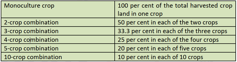
- The curve continues in the same way for other sizes: 6 crops 16.67% each, 7 crops 14.29%, 8 crops 12.5% and 9 crops 11.11%.
- He found the minimum deviation through the standard deviation:
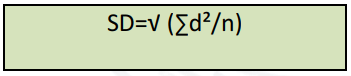
- Here d is the gap between a crop’s actual percentage in a county (areal unit) and its value on the theoretical curve. n counts the crops in that combination.
- Weaver noted that relative, and not absolute, value matters, so he did not extract square roots. The formula actually used is the variance:
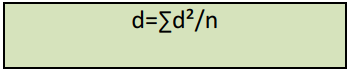
- In this box, the left-hand side stands for the variance, with d inside the sum keeping the meaning given above.
Worked Example: Gorakhpur
- Yearly shares of harvested area: rice 48%, wheat 23%, barley 15%, sugarcane 6% and pulses 5%.
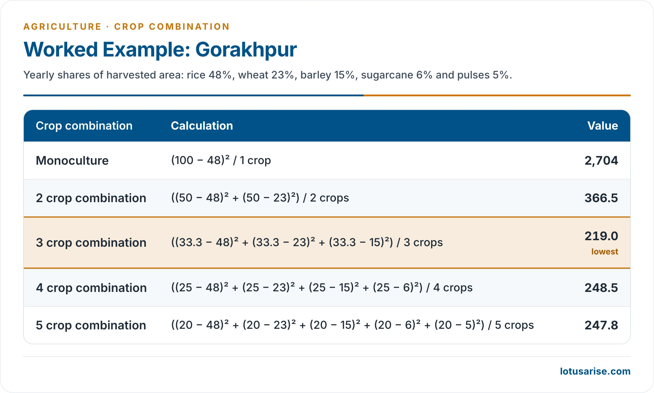
| Combination | Variance |
|---|---|
| Monoculture | 2,704 |
| 2 crops | 366.5 |
| 3 crops | 219.0, the lowest |
| 4 crops | 248.5 |
| 5 crops | 247.8 |
- The deviation from the theoretical curve is lowest for a three-crop combination. Gorakhpur’s basic combination is therefore rice, wheat and barley.
Weaver’s Method Applied to India
- Applied at district level to the data of 2003-06, the technique gives eight-crop combinations for India.
- The pattern that emerges:
- Monoculture of rice: lower Brahmaputra valley, West Bengal, Odisha and coastal Andhra Pradesh.
- Bajra dominant: western Rajasthan.
- Rice and wheat: Punjab and Haryana.
- Wheat, rice and sugarcane: western Uttar Pradesh.
- Four to eight crops: the rest of the country, where wheat, rice, maize, gram, barley, ragi, pulses, oilseeds, cotton, sugarcane, bajra and millets form different associations.
Evaluation of Weaver’s Method
- It has been widely accepted and applied, since it gives a suitable and accurate grouping of crops.
- Its weaknesses:
- It gives unwieldy combinations for units with high crop diversity.
- It involves laborious calculations.
- A crop may occupy little land and yet matter greatly to a region. Weaver handled such a crop by printing its name on the finished map.
- By his own admission, the lowest deviation may sometimes include a crop with as little as one per cent of the cropland.
Modifications of Weaver’s Method
| Worker | Change made |
|---|---|
| Doi (1959) | Replaced the variance with the sum of squared deviations, which simplified the work |
| Peter Scott | Treated animals as equal in importance to crops in Tasmania |
| Thomas (1963) | Brought in data for all crops of a unit when calculating the variance |
| John Terence Coppock (1964) | Converted farm animals to common food units and used the method of least squares |
- Rafiullah (1956) proposed a separate maximum positive deviation method.
- In India, Jasbir Singh (1971) and Singh and Dhillon (1984) made notable contributions.
- Most Indian studies now rest on old data and often cover only crop groups, so a fresh analysis would be useful.
Crop Combination Regions in India
- The method of least squares used by John Terence Coppock in 1964 has been employed to work out India’s crop combination regions.
- Eleven first-ranking crops hold areas large enough to merit separate treatment: rice, wheat, jowar, maize, bajra, ragi, gram, pulses, sugarcane, cotton and oilseeds.
- Another application lists barley, groundnut and tea in place of gram, sugarcane and oilseeds, and recognises 38 combinations.
- First-ranking crops are those with the highest percentage of the cropped area in a component areal unit.
- India is thus divided into 11 crop zones or regions of the first order. These are further divided into dominant crop combination regions, to bring out land use in the transitional areas more meaningfully.
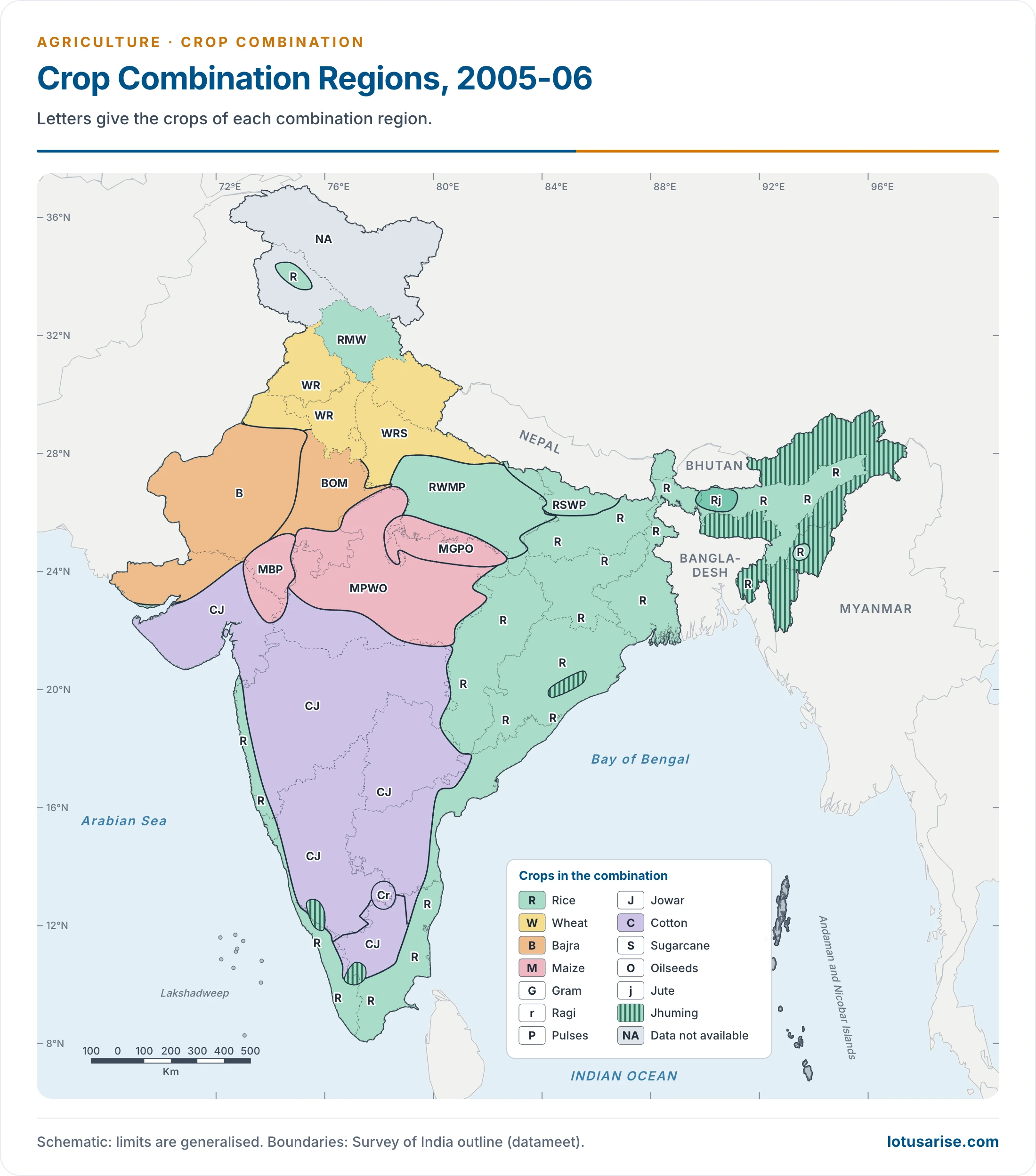
- This map uses the data of 2005-06. Letters give the crops, so that RWMP stands for rice, wheat, maize and pulses, and NA marks units without data.
Generalised Regions by First-Ranking Crop
| First-ranking crop | Main areas | Crops in combination |
|---|---|---|
| Rice | Chhattisgarh, Chotanagpur, West Bengal, Krishna, Godavari and Cauvery deltas, coastal Odisha, Brahmaputra valley, Tripura, Manipur, Nagaland, Andaman and Nicobar Islands (near monoculture) | Few |
| Rice | West coast: Malabar and Konkan | Rubber, coconut, ragi, vegetables, fodder |
| Rice | Non-deltaic east coast: Tamil Nadu, Andhra Pradesh | Groundnut, bajra, jowar, maize |
| Rice | Middle Ganga valley: eastern Uttar Pradesh, Bihar | Wheat, pulses, sugarcane, barley, maize |
| Rice | South Karnataka plateau | Coffee, ragi, pulses, cardamom, coconut, citrus |
| Rice | Jalpaiguri; Meghalaya plateau | Maize; potato, maize, cotton |
| Wheat | Ganga-Yamuna doab, eastern Haryana, Punjab and its foothills | Rice, maize, sugarcane, bajra, pulses, fodder |
| Jowar | Salem-Coimbatore highland, north Karnataka, western and northern Maharashtra, Telangana | Bajra, groundnut, pulses, cotton, rice |
| Maize | South-east Rajasthan with adjoining Madhya Pradesh and Gujarat; hills of Himachal Pradesh and Kashmir | Wheat, rice, groundnut, gram, fodder |
| Bajra | Rajasthan, Kachchh, parts of Uttar Pradesh and Haryana | Wheat, fodder, pulses |
| Ragi | South Karnataka, Dharmapuri | Rice, pulses, groundnut, jowar, coconut |
| Barley | Lahaul-Spiti, Kinnaur | Wheat and hill grains |
| Cotton | Eastern and northern Maharashtra, eastern Gujarat, parts of Madhya Pradesh | Jowar, bajra, groundnut, fodder |
| Groundnut | Anantapur, Kadapa and Chittoor; Kathiawar | Jowar, bajra, dry crops |
| Tea | Darjeeling (near monoculture); Nilgiri | Coffee and vegetables in the Nilgiri |
| Pulses | Uplands south of the Ganga, north-eastern Rajasthan, parts of Odisha, Telangana, Andhra Pradesh | Varies |
- Nowhere in India is wheat a true monoculture. Districts with over 40% of the cropped area under wheat are called wheat regions.
Factors Affecting Crop Combinations
- Three or four crops make up the usual combination, though seven-crop combinations are also common.
- The main factors are physiography, soil fertility, rainfall, weather, irrigation and the farmer’s priorities.
- Irrigation has changed combinations widely in arid and semi-arid tracts.
- Extremes reduce the choice: very dry, very wet, very cold or very hot conditions limit the number of crops.
- Diversity is highest where annual rainfall is about 30–100 cm, and it is also large in the Himalayan hills.
- Combinations form part of the wider study of the cropping pattern of India and feed into agricultural regionalisation.
Previous Year Questions
2013Explain the method of delineating crop-association regions with reference to India.1987Outline the agricultural regions of India indicating the bases of regionalization. Bring out the factors responsible for the emergence of different crop combination in different regions.





Thankyou very much 🙂
This is precise and we’ll organised.
Calculation of sd in monoculture is not correct, it’ll be 2704
there are 23regions according to singh and dhillon based on weaver and cappock scheme
Thanks